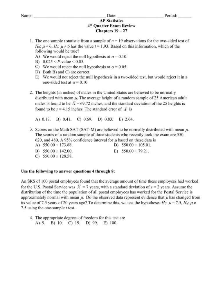
Name: _________________________________ Date: _____________________ Period: ______
AP Statistics
4th Quarter Exam Review
Chapters 19 – 27
1. The one sample t statistic from a sample of n = 19 observations for the two-sided test of
H0:  = 6, Ha:   6 has the value t = 1.93. Based on this information, which of the
following would be true?
A) We would reject the null hypothesis at  = 0.10.
B) 0.025 < P-value < 0.05.
C) We would reject the null hypothesis at  = 0.05.
D) Both B) and C) are correct.
E) We would not reject the null hypothesis in a two-sided test, but would reject it in a
one-sided test at  = 0.10.
2. The heights (in inches) of males in the United States are believed to be normally
distributed with mean . The average height of a random sample of 25 American adult
males is found to be X = 69.72 inches, and the standard deviation of the 25 heights is
found to be s = 4.15 inches. The standard error of X is
A) 0.17.
B) 0.41.
C) 0.69.
D) 0.83.
E) 2.04.
3. Scores on the Math SAT (SAT-M) are believed to be normally distributed with mean .
The scores of a random sample of three students who recently took the exam are 550,
620, and 480. A 95% confidence interval for  based on these data is
A) 550.00 ± 173.88.
D) 550.00 ± 105.01.
B) 550.00 ± 142.00.
E) 550.00 ± 79.21.
C) 550.00 ± 128.58.
Use the following to answer questions 4 through 8:
An SRS of 100 postal employees found that the average amount of time these employees had worked
for the U.S. Postal Service was X = 7 years, with a standard deviation of s = 2 years. Assume the
distribution of the time the population of all postal employees has worked for the Postal Service is
approximately normal with mean . Do the observed data represent evidence that  has changed from
its value of 7.5 years of 20 years ago? To determine this, we test the hypotheses H0:  = 7.5, Ha:  
7.5 using the one-sample t test.
4. The appropriate degrees of freedom for this test are
A) 9. B) 10. C) 19. D) 99. E) 100.
5. The P-value for the one-sample t test is
A) larger than 0.10.
B) between 0.05 and 0.10.
C) between 0.01 and 0.05.
D) below 0.01.
E) impossible to determine, since the standard deviation of the study conducted 20
years ago is not given.
6. A 95% confidence interval for the mean number of years  that a current Postal Service
employee has spent with the Postal Service is
A) 7 ± 2. B) 7 ± 1.984. C) 7 ± 0.4. D) 7 ± 0.3. E) 7 ± 0.2.
7. Suppose the mean and standard deviation we obtained were based on a sample of 25
postal workers, rather than 100. The P-value would be
A) larger.
B) smaller.
C) unchanged, since the difference between X and the hypothesized value  = 7.5 is
unchanged.
D) unchanged, since both groups of workers have the same type of job.
E) unchanged, since the variability measured by the standard deviation stays the same.
8. We wish to see if the dial indicating the oven temperature for a certain model oven is
properly calibrated. Four ovens of this model are selected at random. The dial on each
oven is set to 300° F. After one hour, the actual temperature of each oven is measured.
The temperatures observed are 305°, 310°, 300°, and 305°. Assuming that the actual
temperatures for this model when the dial is set to 300° are normally distributed with
mean , we test whether the dial is properly calibrated by testing the hypotheses
H0:  = 300, Ha:   300. Based on the data, the value of the one-sample t statistic is
A) 5. B) 4.90. C) 2.82. D) 2.45. E) 1.23.
Use the following to answer questions 9 through 11:
Some researchers have conjectured that stem-pitting disease in peach tree seedlings might be
controlled with weed and soil treatment. An experiment was conducted to compare peach tree seedling
growth with soil and weeds treated with one of two herbicides. In a field containing 20 seedlings, 10
were randomly selected from throughout the field and assigned to receive Herbicide A. The remaining
10 seedlings were to receive Herbicide B. Soil and weeds for each seedling were treated with the
appropriate herbicide, and at the end of the study period, the height (in centimeters) was recorded for
each seedling. A box plot of each data set showed no indication of non-normality. The following
results were obtained:
Herbicide A:
Herbicide B:
X 1 = 94.5 cm
X 2 = 109.1 cm
s1 = 10 cm
s2 = 9 cm
9. Referring to the information above, a 95% confidence interval for 2 – 1 is
A) 14.6 ± 7.36. B) 14.6 ± 7.80. C) 14.6 ± 8.95. D) 14.6 ± 13.93.
E) 14.6 ± 33.18.
10. Referring to the information above, suppose we wished to determine if there tended to
be a significant difference in mean height for the seedlings treated with the different
herbicides. To answer this question, we decide to test the hypotheses H0: 2 – 1 = 0,
Ha: 2 – 1  0. Based on our data, the value of the two-sample t test statistic is
A) 14.60. B) 7.80. C) 3.43. D) 2.54. E) 1.14.
11. Referring to the information above, suppose we wished to determine if there tended to
be a significant difference in mean height for the seedlings treated with the different
herbicides. To answer this question, we decide to test the hypotheses H0: 2 – 1 = 0,
Ha: 2 – 1  0. The 90% confidence interval is 14.6 ± 7.80 cm. Based on this
confidence interval,
A) we would not reject the null hypothesis of no difference at the 0.10 level.
B) we would reject the null hypothesis of no difference at the 0.10 level.
C) we would reject the null hypothesis of no difference at the 0.05 level.
D) the P-value is less than 0.10.
E) both C) and D) are correct.
Use the following to answer questions 12 and 13:
An SRS of size 100 is taken from a population having proportion 0.8 of successes. An independent
SRS of size 400 is taken from a population having proportion 0.5 of successes.
12. Referring to the information above, the sampling distribution for the difference in the
sample proportions, p̂1 – p̂2 , has mean
A) equal to the smaller of 0.8 and 0.5.
B) 0.56.
C) 0.3.
D) 0.15.
E) The mean cannot be determined without knowing the sample results.
13. Referring to the information above, the sampling distribution for the difference in the
sample proportions, p̂1 – p̂2 , has standard deviation
A) 1.3. B) 0.40. C) 0.047. D) 0.055. E) 0.002.
Use the following to answer questions 14 and 15:
An SRS of 25 male faculty members at a large university found that 10 felt that the university was
supportive of female and minority faculty. An independent SRS of 20 female faculty found that five
felt that the university was supportive of female and minority faculty. Let p1 represent the proportion
of all male faculty members at the university and p2 represent the proportion of all female faculty
members at the university who hold the stated opinion.
14. Referring to the information above, a 95% confidence interval for p1 – p2 is
A) 0.15 ± 0.355. B) 0.15 ± 0.270. C) 0.15 ± 0.227. D) 0.15 ± 0.138.
E) 0.15 ± 0.168.
15. Referring to the information above, is there evidence that the proportion of male faculty
members who felt the university was supportive of female and minority faculty is larger
than the corresponding proportion for female faculty members? To determine this, you
test the hypotheses H0: p1 = p2, Ha: p1 > p2. The P-value of your test is
A) larger than 0.10.
D) between 0.001 and 0.01.
B) between 0.05 and 0.10.
E) below 0.001.
C) between 0.01 and 0.05.
Use the following to answer questions 16 through 18:
Using computer software, I generate 1000 random numbers that are supposed to follow a standard
normal distribution. I classify these 1000 numbers according to whether their values are less than –2
(value < –2), between –2 and 0 (–2  value < 0), between 0 and 2 (0  value < 2), or at least 2 (value
≥). The results are given in the following table. The expected counts are computed using the 68–95–
99.7 rule.
Observed count
Expected count
Less than
–2
18
25
Between
–2 and 0
492
475
Between
0 and 2
468
475
At least
2
22
25
To test to see if the distribution of observed counts differs significantly from the distribution of
expected counts, we use the χ2 statistic.
16. In this case, the χ2 statistic has approximately a chi-square (χ2) distribution. How many
degrees of freedom does this distribution have?
A) 3. B) 4. C) 7. D) 999. E) 1000.
17. The component (O – E)2/E of the χ2 statistic corresponding to the category “less than 2”
is
A) 0.28.
B) 1.96.
C) 2.72.
D) 3.03.
E) 49.
18. The value of the χ2 statistic is found to be 3.03. The P-value of the test is
A) greater than 0.20.
D) between 0.01 and 0.05.
B) between 0.10 and 0.20.
E) less than 0.01.
C) between 0.05 and 0.10.
19. Which of the following statements is true of chi-square distributions?
A) They take on only positive values.
B) Their density curves are skewed to the left.
C) As the number of degrees of freedom increases, their density curves look more and
more like a uniform distribution.
D) As the number of degrees of freedom increases, their density curves look less and
less like a normal curve.
E) All of the above.
20. Are avid readers more likely to wear glasses than those who read less frequently? Three
hundred men in the Korean army were selected at random and characterized as to
whether they wore glasses and whether the amount of reading they did was above
average, average, or below average. The results are presented in the following table.
Amount of Reading
Above average
Average
Below average
Wear Glasses?
Yes
No
47
26
48
78
31
70
The numerical value of the χ2 statistic for testing the null hypothesis that the amount of
reading you do and whether or not you wear glasses are independent is
A) less than 0.001. B) 2. C) 8.65. D) 21. E) 30.7.
21. Recent revenue shortfalls in a Midwestern state led to a reduction in the state budget for
higher education. To offset the reduction, the largest state university proposed a 25%
tuition increase. It was determined that such an increase was needed simply to
compensate for the lost support from the state. Random samples of 50 freshmen, 50
sophomores, 50 juniors, and 50 seniors from the university were asked whether or not
they were strongly opposed to the increase, given that it was the minimum increase
necessary to maintain the university’s budget at current levels. The results are given in
the following table.
Strongly Opposed?
Yes
No
Freshman
39
11
Year
Sophomore
36
14
Junior
29
21
Senior
18
32
Which hypotheses are being tested by the chi-square test?
A) The null hypothesis is that the closer students get to graduation, the less likely they
are to be opposed to tuition increases. The alternate is that how close a student is to
graduation makes no difference in the student’s opinion.
B) The null hypothesis is that the mean number of students who are strongly opposed
is the same for each of the four years. The alternative is that the mean is different
for at least two of the four years.
C) The null hypothesis is that the distribution of whether or not a student is strongly
opposed is the same for each of the four years. The alternative is that the
distribution is different for at least two of the four years.
D) The null hypothesis is that the distribution of the total number of students sampled
is the same for each of the four years. The alternative is that the distribution is
different for at least two of the four years.
E) The null hypothesis is that a student’s year in school and whether or not the student
is strongly opposed are independent. The alternative is that these variables are
dependent.
Answers:
1. A
2. D
3. A
4. D
5. C
6. C
7. A
8. D
9. C
10. C
11. B
12. C
13. C
14. B
15. A
16. A
17. B
18. A
19. A
20. D
21. C