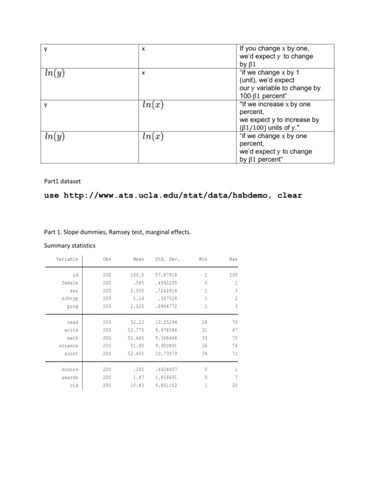
y
If you change x by one,
we’d expect y to change
by β1
“if we change x by 1
(unit), we’d expect
our y variable to change by
100⋅β1 percent”
"If we increase x by one
percent,
we expect y to increase by
(β1/100) units of y."
“if we change x by one
percent,
we’d expect y to change
by β1 percent”
x
x
y
Part1 dataset
use http://www.ats.ucla.edu/stat/data/hsbdemo, clear
Part 1. Slope dummies, Ramsey test, marginal effects.
Summary statistics
Variable
Obs
Mean
Std. Dev.
Min
Max
id
female
ses
schtyp
prog
200
200
200
200
200
100.5
.545
2.055
1.16
2.025
57.87918
.4992205
.7242914
.367526
.6904772
1
0
1
1
1
200
1
3
2
3
read
write
math
science
socst
200
200
200
200
200
52.23
52.775
52.645
51.85
52.405
10.25294
9.478586
9.368448
9.900891
10.73579
28
31
33
26
26
76
67
75
74
71
honors
awards
cid
200
200
200
.265
1.67
10.43
.4424407
1.818691
5.801152
0
0
1
1
7
20
. regress read c.math##c. socst
Source
SS
df
MS
Model
Residual
11424.7622
9494.65783
3
196
3808.25406
48.4421318
Total
20919.42
199
105.122714
Std. Err.
Number of obs
F( 3,
196)
Prob > F
R-squared
Adj R-squared
Root MSE
t
P>|t|
=
=
=
=
=
=
200
78.61
0.0000
0.5461
0.5392
6.96
read
Coef.
[95% Conf. Interval]
math
socst
-.1105123
-.2200442
.2916338
.2717539
-0.38
-0.81
0.705
0.419
-.6856552
-.7559812
.4646307
.3158928
c.math#c.socst
.0112807
.0052294
2.16
0.032
.0009677
.0215938
_cons
37.84271
14.54521
2.60
0.010
9.157506
66.52792
Remark: reading score, math score, social science score
1. Write out the estimated equation, use e to denote the error term.
̂0 + 𝛽
̂1 𝑥1 + 𝛽
̂2 𝑥2 + 𝛽
̂3 𝑥1 × 𝑥2 + 𝑒
𝑦̂ = 𝛽
2. Is the estimated coefficient significant at 5% level? Use 3 ways to illustrate your result based on
the regression table above. You don’t have to write out the critical t value, but say how to
display it on Stata.
t- value, p-value, 95%CI
t-value= display invttail(196,0.025) since it is a two sided test.
3.
a. Explain what the coefficient for the interaction here means.
The estimated coefficient (effect) of math on reading changes by 0.0112807 if socst
increases by 1 unit.
b. Given math=50, what is the effect of socst on read
i. take derivative of the estimated equation with respect to socst, then, plug in 50
for math.
c. Given socst= 30, what is the effect of math on read
Here is a Ramsey test of the regression above
F(3, 193) =
Prob > F =
1.12
0.3432
State the Null for Ramsey and whether you reject at 5% level.
H_0: the model has no omitted variables.
Note that this is different from the overall test, which has null: b_1=b_2=… =0
y here is “read”
Average marginal effects
Model VCE
: OLS
Number of obs
=
200
Expression
: Linear prediction, predict()
ey/ex w.r.t. : math
ey/ex
math
Delta-method
Std. Err.
.7260325
.059477
z
12.21
P>|z|
[95% Conf. Interval]
0.000
.6094598
.8426053
. margins, eyex( math) atmeans
Conditional marginal effects
Model VCE
: OLS
Number of obs
=
200
Expression
: Linear prediction, predict()
ey/ex w.r.t. : math
at
: math
=
52.645 (mean)
Delta-method
ey/ex
Std. Err.
math
.730566
.0592294
z
12.33
P>|z|
[95% Conf. Interval]
0.000
.6144786
.8466534
Compare the tables above, what can you conclude about this dataset.
To answer this type of question, you should not use words that are affirmative such as must be, should
be, definitely, etc. You don’t see the data, or the whole distribution of elasticity. Explain what you see
first, and then try to interpret what might be going on.
a. Point out the difference between ave elasticity and elasticity at ave.
b. The two values are not far away from each other, which indicates there is no tremendous
change in the trend of the elasticity. We showed this before ( such as a u shape or wedge shape
trend). It might be linear, but we don’t know.
c. Note that the margin at ave is slightly higher than the ave margin. This means that there might
be more weight in the lower tail of math score distribution.
Part2, regression, testing and prediction and forecasting
Dataset for part2
use http://www.ats.ucla.edu/stat/stata/webbooks/reg/elemapi2, clear
Api00(academic performance in 2000)
1. Complete the table above.
Apply the formulas for the most.
Note that: this is only true for numerator df =1 for the F. Namely, you only have 1 independent variable.
F= t^2
You get t, then std. Err is just t/4.554; because the default testing is whether estimated coefficient is
significant. i.e H_0: \beta =0
. regress api00 ell meals yr_rnd mobility acs_k3 acs_46 full emer enroll
Source
SS
df
MS
Model
Residual
6740702.01
1240707.78
9
385
748966.89
3222.61761
Total
7981409.79
394
20257.3852
api00
Coef.
ell
meals
yr_rnd
mobility
acs_k3
acs_46
full
emer
enroll
_cons
-.8600707
-2.948216
-19.88875
-1.301352
1.3187
2.032456
.609715
-.7066192
-.012164
758.9418
Std. Err.
.2106317
.1703452
9.258442
.4362053
2.252683
.7983213
.4758205
.6054086
.0167921
62.28601
t
-4.08
-17.31
-2.15
-2.98
0.59
2.55
1.28
-1.17
-0.72
12.18
Number of obs
F( 9,
385)
Prob > F
R-squared
Adj R-squared
Root MSE
P>|t|
0.000
0.000
0.032
0.003
0.559
0.011
0.201
0.244
0.469
0.000
=
=
=
=
=
=
395
232.41
0.0000
0.8446
0.8409
56.768
[95% Conf. Interval]
-1.274203
-3.28314
-38.09219
-2.158995
-3.110401
.462841
-.3258169
-1.89694
-.0451798
636.4785
-.4459382
-2.613293
-1.685309
-.4437088
5.747801
3.602071
1.545247
.4837019
.0208517
881.4051
2. Is the overall test significant at 5%?
3. Is each coefficient significant at 5%?
Variable
Obs
Mean
Std. Dev.
Min
Max
snum
dnum
api00
api99
growth
400
400
400
400
400
2866.81
457.735
647.6225
610.2125
37.41
1543.811
184.8231
142.249
147.1363
25.24739
58
41
369
333
-69
6072
796
940
917
134
meals
ell
yr_rnd
mobility
acs_k3
400
400
400
399
398
60.315
31.4525
.23
18.25313
19.1608
31.9117
24.83919
.4213595
7.484563
1.368693
0
0
0
2
14
100
91
1
47
25
acs_46
not_hsg
hsg
some_col
col_grad
397
400
400
400
400
29.68514
21.2525
26.015
19.7125
19.6975
3.840784
20.67577
16.33269
11.33694
16.47071
20
0
0
0
0
50
100
100
67
100
grad_sch
avg_ed
full
emer
enroll
400
381
400
400
400
8.6375
2.668478
84.55
12.6575
483.465
12.13091
.7637868
14.94979
11.74649
226.4484
0
1
37
0
130
67
4.62
100
59
1570
mealcat
collcat
400
400
2.015
2.02
.8194227
.816251
1
1
3
3
4. Calculate beta coefficients for ell and meals
Standardized beta = b * sd(x)/sd(y)
5. Note that yr_rnd is a dummy variable indicating whether the person is in year round school.
Api00 is the academic performance index. Explain what the estimated coefficient means, and is it
significant?
6. Keep others constant, how much change in acs_46 would result one standard deviation change in
api00.
. set obs 401
obs was 400, now 401
. replace ell = 50 in 401
(1 real change made)
. replace meals = 40 in 401
(1 real change made)
. replace yr_rnd = 0 in 401
(1 real change made)
. replace mobility = 25 in 401
(1 real change made)
. replace acs_k3 = 19 in 401
(1 real change made)
. replace acs_46 = 30 in 401
(1 real change made)
. replace full = 90 in 401
(1 real change made)
. replace emer = 8 in 401
(1 real change made)
. replace enroll = 300 in 401
(1 real change made)
The predicted SE is predicSE
9.977622
Predict what the 95% CI for the x given above
Forecast what the 95% CI (you should know how to calculate forecast SE based on the known info)
Plug the observation into the estimated equation, get the conditional mean.
PredicSE^2 + Root MSE^2 = ForecastSE^2
Then build the CI.
7. If you want to test the coefficient for meals has a negative effect.
a. Set up your H0 and Ha
b. What is your p-value here
c. Do you reject it at 1% significance level.
8. This is your dataset, calculate the OLS
88.00
12
80.00
6
96.00
8
95.00
85.00
91.00
93.00
83.00
90.00
5
7
5
7
6
8