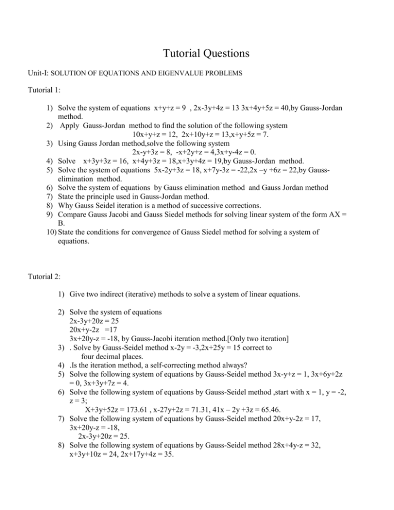
Tutorial Questions
Unit-I: SOLUTION OF EQUATIONS AND EIGENVALUE PROBLEMS
Tutorial 1:
1) Solve the system of equations x+y+z = 9 , 2x-3y+4z = 13 3x+4y+5z = 40,by Gauss-Jordan
method.
2) Apply Gauss-Jordan method to find the solution of the following system
10x+y+z = 12, 2x+10y+z = 13,x+y+5z = 7.
3) Using Gauss Jordan method,solve the following system
2x-y+3z = 8, -x+2y+z = 4,3x+y-4z = 0.
4) Solve x+3y+3z = 16, x+4y+3z = 18,x+3y+4z = 19,by Gauss-Jordan method.
5) Solve the system of equations 5x-2y+3z = 18, x+7y-3z = -22,2x –y +6z = 22,by Gausselimination method.
6) Solve the system of equations by Gauss elimination method and Gauss Jordan method
7) State the principle used in Gauss-Jordan method.
8) Why Gauss Seidel iteration is a method of successive corrections.
9) Compare Gauss Jacobi and Gauss Siedel methods for solving linear system of the form AX =
B.
10) State the conditions for convergence of Gauss Siedel method for solving a system of
equations.
Tutorial 2:
1) Give two indirect (iterative) methods to solve a system of linear equations.
2) Solve the system of equations
2x-3y+20z = 25
20x+y-2z =17
3x+20y-z = -18, by Gauss-Jacobi iteration method.[Only two iteration]
3) . Solve by Gauss-Seidel method x-2y = -3,2x+25y = 15 correct to
four decimal places.
4) .Is the iteration method, a self-correcting method always?
5) Solve the following system of equations by Gauss-Seidel method 3x-y+z = 1, 3x+6y+2z
= 0, 3x+3y+7z = 4.
6) Solve the following system of equations by Gauss-Seidel method ,start with x = 1, y = -2,
z = 3;
X+3y+52z = 173.61 , x-27y+2z = 71.31, 41x – 2y +3z = 65.46.
7) Solve the following system of equations by Gauss-Seidel method 20x+y-2z = 17,
3x+20y-z = -18,
2x-3y+20z = 25.
8) Solve the following system of equations by Gauss-Seidel method 28x+4y-z = 32,
x+3y+10z = 24, 2x+17y+4z = 35.
9) Solve the following system of equations by Gauss-Seidel method 6x+3y+12z = 35, 8x3y+2z = 20, 4x+11y-z = 33.
10) Solve the following system of equations by Gauss-Seidel method 8x-y+z = 18, 2x+5y-2z
= 3, x+y-3z = -6.
Tutorial 3:
1. Find the inverse of the coefficient matrix by Gauss-Jordan elimination method.
5x-2y = 10
3x+4y = 12.
2. Define Gauss Elimination method
3. State the principle used in Gauss-Jordan method.
4. ……………. Method,the values are get immediately without using the process of back
substitution.
y=1,2 . Find the marginal distribution
5) Explain the procedure for method of triangularization
6) Solve the following system of equations by Gauss elimination method
x+y+54z = 110
27x+6y-z = 85
6x+15y+2z = 72.
7) Solve the following system of equations
2x+3y-z = 5
4x+4y-3z = 3
2x-3y+2z = 2, by method of factorization
8) Solve the following system by triangularization method
X+y+z=1 ; 4x+3y-z=6 ; 3x+5y+3z=4
9) Solve the following system by triangularization method
3x1-x2 =-5 ; - x1+3x2 –x3 =10: - x2+3x3 –x4 =-15:
- x3+3x4 =15
10) Solve the following system by crout’smethod
2x-y+8z=24 : 5x+4y-3z=2 ;3x+y+2z=16
Unit-II: INTERPOLATION AND APPROXIMATION
Tutorial 1:
1. Construct a linear interpolating polynomial given the points (x0,y0) and (x1,y1).
2. Using Lagranges find y at x = 2 for the following
X: 0
1
3
4
5
Y:
0
1
81
256
625
3. Explain the use of Lagrange’s interpolation formula.
4. Obtain the Lagrange’s interpolating polynomial for the observed data of points (1,1),(2,1)
and (3,-2).
5) Using Lagrange’s interpolation ,find y(2) from the following data:
x
y
0
0
1
1
3
81
4
256
5
625
6) Using Lagrange’s interpolation formula,compute f(4); given
f(0)=2,f(1)=3,f(2)=12,f(15)=3587.
7) Using Lagrange’s interpolation formula,compute y(10); given
y(5)=12,y(6)=13,y(9)=14,y(11)=16.
8) Using Lagrange’s formula fit a polynomial to the data
x
y
-1
7
1
5
2
15
9) Find the missing term in the following table using Lagrange’s interpolation:
x
y
0
1
1
3
2
9
3
-
4
81
10) Find the Lagrangian interpolating polynomial for the following data:
x
f(x)
1
0
2
7
3
26
5
124
Tutorial 2:
1) State the conditions required for a natural cubic spline.
2) State the order of convergence of cubic spline.
3) Find the cubic spline for the following data
X: 0
2
4
6
Y: 1
9
21
41
4) State Newton’s forward and backward interpolating formula.
5) Using Lagrange’s formula,prove
y1 = y3-0.3(y5- y-3)+0.2(y-3-y-5) nearly.
6) From the data given below.Find the value of x when y = 13.5
x
y
93
96.2
11.38 12.8
100.0
14.7
104.2
17.07
108.7
19.91
7) Apply Lagrange’s formula to find theroot of the equation f(x) = 0 given that f(30)=30,f(34) = -13,f(38) = 3,f(42) = 18.
8) Using Newton’s divided difference,find u(3) given u(1) = -26,u(2) = 12, u(4) = 256,
(6) = 844.
u
9) Using Newton’s divided difference formula, find the values of f(2), and f(12) from the
given table:
x : 4
5
7
10
11
13
f(x) : 48
100 294 900 1210 2028
10) From the following table find f(x) and hence f(6) using Newton’s forward interpolation
formula
x
f(x)
1
1
2
5
7
5
8
4
Tutorial 3:
1) Given data
X: 0
1
2
4
Y: 0
3
4
8 find y at x=3 using lagrange’s formula
2) Using striling’s formula to find y35 from the following
X: 20
30
40
50
Y: 512
439
346
243
3) What is the lagrange’s formula to find y, if there sets of values (x0,y0), (x1,y1) and
(x2,y2) are given
4) Write the cubic spline formula
5) Using Newton’s forward interpolation formula,find the polynomial f(x) satisfying the
following data.Hence find y at x = 5
x
:
4
6
8
10
y :
1
3
8
16
6) A third degree polynomial passes through the points (0,-1),(1,1),(2,1) and (3,-2)
using Newton’s forward interpolation formula,find the polynomial. Hence find the
value at 1.5.
7) Use Newton’s backward difference formula to construct an interpolating polynomial
of degree 3 for the data:
F(-0.75) = - 0.07181250, f(-0.5) = -0.024750, f(-0.25) = 0.33493750, f(0) =
1.10100.Hence find f(-1/3).
8) The following data are taken from the steam table: Find the pressure at temperature t
= 1420 and t = 1750.
Temp.0C
140
150
160
170
180
Pressure
3.685 4.854 6.302 8.076 10.225
2
kgf/cm
9) From the following table,find thevalue of tan 45015’ by Newton’s forward
interpolation formula.
x0
45 46
47
48
49
50
tan x 0 1
1.03553 1.07237 1.11061 1.15037 1.191175
10) From the following table,of half-yearly premium for policies maturing at different
ages,estimate the premium for policies maturing at age 46 and 63.
Age x
45
50
Premium y
114.84 96.16
55
60
65
83.32
74.48
68.48
Unit-III: NUMERICAL DIFFERENTIATION AND INTEGRATION
Tutorial 1:
1) Using Newton’s backward difference formula, write the formula for the first and second
derivatives at the end values x=𝑥𝑛 up to the forth order difference term.
2) In numerical integration, what should be the number of intervals to apply Simpson’s 1/3
rule and by Simpson’s 3/8 rule?
3) Compare Trapezoidal rule and Simpson’s 1/3 rule for evaluating numerical integration.
4) Why is Trapezoidal rule so called?
5) The following data gives the velocity of a particle for 20 seconds at
an interval of 5seconds.Find the initial acceleration using the entire
data.
Time(sec)
0
5
10
15
20
Velocity(m/sec) 0
3
14
69
6) Find the maximum and minimum value of y tabulated below.
228
x
-2
-1
0
1
2
3
4
y
2
-0.25
0
-0.25
2
15.75 56
7) Consider the following table of data:
x
0.2
0.4
0.6
0.8
1.0
F(x) 0.9798652 0.9177710 0.8080348 0.6386093 0.3843735
Find 𝑓 0.25)using Newton’s forward difference approximation. 𝑓 ′ (0.6)
using Stirling’s approximation and 𝑓 ′ (0.95) using Newton’s backward
difference approximation.
8) Obtain the value of f(0.15) using Stiriling’s formula given in the
table below.
′(
x
f(x)
0.10
0.20
0.30
0.40
0.50
0.60
0.1023 0.1047 0.1071 0.1096 0.1122 0.1148
9) Given the following data,find y’(6) and the maximum value of y
x : 0
2
3
4
7
9
y:
4
26
38 112 466 922
10) The table given below reveals the velocity v of a body during the time “t” specified.Find
its acceleration at t = 1.1.
t :
V :
1.0 1.1
43.1 47.7
1.2 1.3
52.1 56.4
1.4
60.8
Tutorial 2:
When does Simpson’s rule give exact result?
State Simpson’s 3/8 rule
What is the local error term inTrapezoidal formula and in Simpson’s one third rule?
For what type of functions,Simpson’s rule and direct integration will give the same
result?
1 𝑑𝑥
5. mEvaluate ∫0 1+𝑥 2 with h = 1/6 by Trapezoidal rule.
1.
2.
3.
4.
2 𝑑𝑥
6. Evaluate the integral ∫1
1+𝑥 2
, using Trapezoidal rule with two sub-intervals.
𝜋/2
7. Dividing the range into 10 equal parts, find the value of ∫0 𝑠𝑖𝑛𝑥 𝑑𝑥,by
(i) Trapezoidal rule (ii) Simpson’s rule.
1
8. Using Simpson’s rule one third rule evaluate ∫0 𝑥 𝑒 𝑥 dx taking 4 intervals. Compare
your result with actual value.
0.7
9. Calculate ∫0.5 𝑒 −𝑥 √𝑥 dx ,taking 5 ordinates by Simpson’s rule.
𝜋/2
10. Using Trapezoidal rule evaluate ∫0
√𝑠𝑖𝑛𝑥 dx.
Tutorial 3:
𝑏
1. State Trapezoidal rule for evaluating ∫𝑎 ∫𝑑 𝑓(𝑥, 𝑦) 𝑑𝑥 𝑑𝑦.
𝑐
𝑏
2. State Simpson’s rule for evaluating ∫𝑎 ∫𝑑 𝑓(𝑥, 𝑦) 𝑑𝑥 𝑑𝑦.
𝑐
3. State Newton’s formula to find f’(x), f’’(x) and f’’’(x) using forward difference
𝑑𝑦
4. Find 𝑑𝑥 at x=1 from the table
X: 1
2
3
4
f(x):1
8
27
64
1
2
5. Obtain the approximate value of∫−1 𝑒 −𝑥 cosxdx using Lobatto integration method
2
2
6. Evaluate ∫1 ∫1
1
𝑥 2 +𝑦 2
𝑑𝑥 𝑑𝑦 𝑢𝑠𝑖𝑛𝑔 Trapezoidal rule with h=0.2 & k=0.25
(or)
7. Derive the Trapezoidal rule formula for double integration
1.4
2.4 1
8. Evaluate ∫1 ∫2
𝑥𝑦
𝑑𝑥 𝑑𝑦 𝑢𝑠𝑖𝑛𝑔 Trapezoidal and Simpson’s rule and verify your result
by actual integration
1
2
9. Evaluate ∫0 ∫1
10.
2𝑥𝑦
(1+𝑥 2 )(1+𝑦 2 )
𝑑𝑥 𝑑𝑦 𝑢𝑠𝑖𝑛𝑔 Trapezoidal rule with h= & k=0.25
Derive simpson’s rule for double integration
Unit-IV: INITIAL VALUE PROBLEMS FOR ORDINARY DIFFERENTIAL EQUATIONS
Tutorial 1:
𝑑𝑦
1) Solve the differential equation 𝑑𝑥 = x+y +xy ,y(0) =1,by Taylor’s method to get the
value of y at x = h?
2) What is the truncation error in Taylor’s series?
3) By Taylor series, find y(1.1) given y  = x + y, y(1) = 0.
4) Find the Taylor series up to x3 term satisfying 2 y   y  x  1, y (0)  1 .
5) Using Taylor series method,find y(1.1) and y(1.2) given 𝑦 ′ = x+y, y(1) = 0.
𝑑𝑦
6) Find the Taylor series solution with three terms for the initial value problem 𝑑𝑥 =
𝑥 3 +y,
y(1) = 1.
𝑑𝑦
7) Using Taylor’s series method with the first five terms in the expansion = 𝑒 𝑥 -𝑦 2 ,y(0)
𝑑𝑥
= 1.
8) Using Taylor’s series method,compute y(0.2) and y(0.4) correct to 4 decimal places
𝑑𝑦
given
=1-2xy and y(0) = 0.
𝑑𝑥
9) Solve 𝑦 ′ =y2+x,y(0) = 1,find y(0.2) and y(0.4) by Taylor’s series method.
10) Given 𝑦 ′ − 2𝑦 = 3ex,y(0) = 0,compute y for x = 0.1(0.1)0.2 by Taylor’s series method.
Tutorial 2:
1. Using Euler’s method find the solution of the IVP
dy
 log( x  y ), y (0)  2 at
dx
x  0.2 taking h  0.2 .
𝑑𝑦
2. Using modified Euler’s method find y(0.1) if 𝑑𝑥 = 𝑥 2 +𝑦 2 ,y(0) = 1.
3. Write the Runge-Kutta algorithm of second order for solving y’ = f(x,y), y(x0)=y0.
4. Write the Runge-Kutta algorithm of second order for solving y’ = f(x,y), y(x0)=y0.
5. Evaluate the values of y(0.1) and y(0.2) given 𝑦 ′′ -x(𝑦 ′ )2 +y2 = 0; y(0) = 1, 𝑦 ′ (0) = 0
by using Taylor’s series method.
6. Solve 𝑦 ′′ = y+x𝑦 ′ , y(0) = 1, 𝑦 ′ (0) = 0, by Taylor’s series method.
𝑑𝑦
𝑦−𝑥
7. Given 𝑑𝑥 = 𝑦+𝑥, with the boundary condition y=1 for x = 0,find y(0.1) by Euler’s
method.
𝑑𝑦
8. Use Euler’s method find y(0.2) and y(0.4) from 𝑑𝑥 = x+y, y(0) = 1 with h = 0.2.
9. Using Euler’s method solve 𝑦 ′ = x+y+xy, y(0) = 1. Compute y at x = 0.1 ,by taking h
= 0.05.
𝑑𝑦
1
10. Using Euler’s method find y(0.3) of y(x) satisfies the initial value problem 𝑑𝑥 = 2 (𝑥 2 +
1)𝑦 2 , y(0.2) = 1.1114.
Tutorial 3:
1. Is Euler’s method formula ,a particular case of second order Runge-Kutta method?
2. The fourth order Runge- Kutta Methods are used widely in………..of differential
equations.
3. State Adams – Bash forth predictor and corrector formula.
4. What is the condition to apply Adams – Bash forth method
5. Write Milne’s predictor corrector formula.
𝑑𝑦
6. Given 𝑑𝑥 =x3+y, y(0) =2,y(0.2)= 2.073,y(0.4) = 2.452, y(0.6) = 3.023. Compute y(0.8) by
Milne’s predictor corrector method by h = 0.2.
𝑑𝑦
2𝑥𝑦
7. Using Runge-Kutta method calculate y(0.1), y(0.2)and y(0.3) given that 𝑑𝑥 - 1+𝑥 2 = 1,
y(0) =0.Taking these values as starting values find y(0.4) by Milne’s method.
8. Solve 𝑦 ′ =x2+y2-2 ,using Milne’s method for x = 0.3 given
x
y
9. Solve 𝑦 ′ = y -
-0.1
1.09
2𝑥
𝑦
0
1
0.1
0.89
0.2
0.7605
, y(0) =1,y(0.1) = 1.0954,y(0.2) = 1.1832,y(0.3)=1.2649,find y(0.4) by
Adam’s method.
𝑑𝑦
10. Find y(0.1), y(0.2),y(0.3) from 𝑑𝑥 = xy +y2 ,y(0) = 1 by using Runge-Kutta method and
hence obtain y(0.4) using Adam’s method.
Unit-V: BOUNDARY VALUE PROBLEMS IN ORDINARY AND PARTIAL
DIFFERENTIAL EQUATIONS
Tutorial 1:
1. What is the classification of fx-fyy=0?
2. Give an example of a parabolic equation?
3. Give an example of a parabolic equation?
4.State Schmidt’s explicit formula for sloving heat flow equation?
5.Solve 𝑦 ′′ -xy = 0 given y(00 =-1 , y(1) = 2 by finite difference method taking n = 2.
1 2
6.Solve the equation 𝑦 ′′ (x)-xy(x) = 0 , for every y(𝑥𝑖 ), 𝑥𝑖 = 0, 3 , 3 , 𝑔𝑖𝑣𝑒𝑛 𝑡ℎ𝑎𝑡 𝑦(0) +
𝑦 ′ (0) =1 and y(1) = 1, by finite difference method.
𝜕𝑢
𝜕2 𝑢
7.Solve 𝜕𝑡 = 𝜕𝑥 2 , 0≤x≤1, t≥0 with u(x,0) = x (1-x), 0<x<1 and u(0,t) = u(1,t) =0, for all t>0
using explicit method with ∆𝑥 = 0.2 for 3 time steps.
8.Solve 𝑢𝑥𝑥 = 32𝑢𝑡 , taking = 0.25 for t>0 , 0<x<1 and u(x,0) = 0 , u(0,t) = 0, u(1,t) = t.
9. Solve 𝑢𝑡 = 𝑢𝑥𝑥 , subject to u(0,t) = u(1,t) =0 and u(x,0) =sinπx , 0<x<1
10. Find the values of the function u(x,t) satisfying the differential equation 𝑢𝑡 = 4 𝑢𝑥𝑥
and the boundary condition u(0,t) = u(8,t) =0 and
u(x,0) = 4x-
1
𝑥2
2
at the point x
= I, I = 0,1,2,3,4 and t = 8j , j =0,1,2,3,4,5.
Tutorial 2:
1. Write down the implicit formula to solve one dimensional heat flow equation
𝑢𝑥𝑥 =
1
𝑢.
𝑐2 𝑡
2. Why is Crank- Niholson scheme called an implicit scheme?
3. Write the Crank Nicholson difference scheme to solve uxx=aut with u(0,t) = T0,
u(l,t)=T1 and the initial condition as u(x,0) = f(x)?
4. Write a note on the stability and convergence of the solution of the difference equation
corresponding to the hyperbolic equation utt=a2 uxx.
5. For what purpose Bender-Schmidt recurrence relation is used? Solve by CrankNicolson’s method the equation 𝑢𝑥𝑥 = 𝑢𝑡 , subject to u(x,0) = 0 , u(0,t) = 0 and u(1,t) = t ,
for two time steps.
6. Solve 𝑦𝑡𝑡 = 𝑦𝑥𝑥 up to t = 0.5 with a spacing of 0.1 subject to y(0,t) = 0, y(1,t) = 0 , 𝑦𝑡 (x,0)
= 0 and y(x,0) = 10+ x(1-x).(wave equation)
𝜕2 𝑢
𝜕2 𝑢
7. Approximate the solution to the wave equation 𝜕𝑥 2 = 𝜕𝑡 2 , 0 < 𝑥 < 1, 𝑡 > 0, u(0,t) = 0,
u(1,t) = 0, t>0,
u(x, 0) = sin2πx, 0≤x≤1 with∆𝑥 = 0.25 𝑎𝑛𝑑 ∆𝑡 = 0.25 𝑓𝑜𝑟 𝑡ℎ𝑟𝑒𝑒 𝑡𝑖𝑚𝑒 𝑠𝑡𝑒𝑝𝑠.
𝜕2 𝑢
𝜕2 𝑢
𝜕2 𝑢
𝜕2 𝑢
8. Solve 𝜕𝑡 2 = 𝜕𝑥 2 , 0 < 𝑥 < 1, 𝑡 > 0,
given u(x,0) = 𝑢𝑡 (x,0) = u(0,t)=0 and u(1,t) = 100 sin πt.
Compute u for 4 times stpes with h = 0.25.
𝜕𝑢
9. Solve 𝜕𝑡 2 = 𝜕𝑥 2 , 0 < 𝑥 < 1, 𝑡 > 0, u(0,t) = u(1,t) = 0, u(x,0) = x- x2, 𝜕𝑡 (x,0) = 0 taking h
= 0.2 upto one half of the period of vibration by taking appropriate time step.
10. Solve
0.
Tutorial 3:
𝜕2 𝑢
𝜕𝑡 2
=
𝜕2 𝑢
𝜕𝑥 2
, 0 < 𝑥 < 1, 𝑡 > 0, u(x,0) = 100(x- x2) , 𝑢𝑡 (x,0) = 0, u(0,t) = 0, u(1,t) =
1. Using Crank-Nicolson’s Implicit scheme , Solve 16𝑢𝑡 = 𝑢𝑥𝑥 , 0<x<1, t>0, given that u(x,0 )
=0 , u(0,t) = 0, u(1,t) = 100t.
𝜕𝑢
𝜕2 𝑢
2. Using Crank-Nicolson’s Implicit scheme Solve 𝜕𝑡 = 𝜕𝑥 2 , u(x,0) = u(0,t) = 0 , u(1,t) = t ,
choosing h = 0.5 , k = 1/8.
3. Solve 𝑢𝑡 = 5𝑢𝑥𝑥 , u(0,t) = 0, u(5,t) = 60 , u(x,0) = 20x ; 0≤x≤3 = 60 ; 3≤x≤5, using
explicit finite difference scheme , choosing h = 1.
𝜕𝑢
𝜕2 𝑢
4. Solve 𝜕𝑡 = 𝜕𝑥 2 , 0 < 𝑥 < 5 , 𝑡 > 0, given that u(x,0) = 20, u(0,t) = 0, u(5,t) = 100. Compute
u for one time step with h = 1 by Crank-Nicolson’s method.
𝜕2 𝑢
𝜕𝑢
𝜋𝑥
5. Solve 𝜕𝑥 2 = 𝜕𝑡 , 0 < 𝑥 < 2, 𝑡 > 0, u(0,t) = u(2,t) = 0, t>0 and u(x,0) = sin 2 , 0≤x≤2 using h
=0.5, k=0.25 for two time steps by Crank-Nicolson’s method.
𝜕𝑢
𝜕2 𝑢
6. Solve 𝜕𝑡 = 𝜕𝑥 2 , subject to the conditions u(x,o) = sinπx , 0≤x≤1 , u(0,t) = u(1,t) = 0 ; using
Crank-Nicolson’s method taking h =1/3 , k = 1/36.
7. State the general form of Poisson’s equation in partial derivatives?
8. Define the local truncation error.
9. Derive Crank-Niclson scheme.
10. What is the error for solving Laplace and Poissson’s equation by finite difference method?