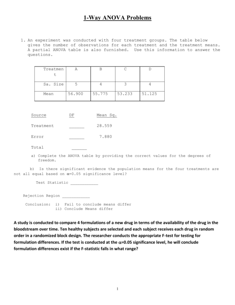
1-Way ANOVA Problems
1. An experiment was conducted with four treatment groups. The table below
gives the number of observations for each treatment and the treatment means.
A partial ANOVA table is also furnished. Use this information to answer the
questions.
Treatmen
t
A
B
C
D
Sa. Size
5
4
3
4
56.900
55.775
53.233
51.125
Mean
Source
DF
Mean Sq.
Treatment
______
28.559
Error
______
7.880
Total
______
a) Complete the ANOVA table by providing the correct values for the degrees of
freedom.
b) Is there significant evidence the population means for the four treatments are
not all equal based on =0.05 significance level?
Test Statistic ____________
Rejection Region ____________
Conclusion:
i) Fail to conclude means differ
ii) Conclude Means differ
A study is conducted to compare 4 formulations of a new drug in terms of the availability of the drug in the
bloodstream over time. Ten healthy subjects are selected and each subject receives each drug in random
order in a randomized block design. The researcher conducts the appropriate F-test for testing for
formulation differences. If the test is conducted at the =0.05 significance level, he will conclude
formulation differences exist if the F-statistic falls in what range?
1
A study is conducted to compare golf ball distances among 4 brands of golf balls. A mechanical driver is set
up and hits 12 balls of each brand, and the distance travelled (meters) is measured. The F-test determines
that there are differences among the brands. A follow-up comparison based on Tukey’s method yields the
following table:
Multiple Comparisons
Dependent Variable: y
Tukey HSD
(I) group
1
(J) group
2
3
4
1
3
4
1
2
4
1
2
3
2
3
4
Mean
Difference
(I-J)
St d. E rror
-21.40796*
2.51529
-.00121
2.51529
-12.43549*
2.51529
21.40796*
2.51529
21.40675*
2.51529
8.97247*
2.51529
.00121
2.51529
-21.40675*
2.51529
-12.43428*
2.51529
12.43549*
2.51529
-8. 97247*
2.51529
12.43428*
2.51529
Sig.
.000
1.000
.000
.000
.000
.005
1.000
.000
.000
.000
.005
.000
95% Confidenc e Int erval
Lower Bound Upper Bound
-28.1238
-14.6921
-6. 7171
6.7146
-19.1513
-5. 7196
14.6921
28.1238
14.6909
28.1226
2.2566
15.6883
-6. 7146
6.7171
-28.1226
-14.6909
-19.1501
-5. 7184
5.7196
19.1513
-15.6883
-2. 2566
5.7184
19.1501
*. The mean difference is significant at the .05 level.
Clearly state what can be said of all pairs of brands at the 0.05 experimentwise error rate.
Brands:
1 vs 2:
1 vs 3:
1 vs 4:
2 vs 3:
2 vs 4:
3 vs 4:

A comparison of 3 drugs was conducted to test whether there are any differences among their effects of
relieving pain. The mean relief ratings and standard deviations are given below. Each drug was assigned at
random to 10 subjects in a completely randomized design (n1=n2=n3=10).
Drug
Mean
SD
1
8
1
2
10
2
3
12
2
o
o
o
o
H0: Not all i are equal
Between Drug Sum of Squares and degrees of freedom:
Within Drug Sum of Squares and degrees of freedom:
F-Statistic _______________________________
Reject H0 (at =0.05 level) if F-statistic is Above / Below ____________
2
Ford wants to compare mean assembly times for Explorer’s at their 3 assembly plants. They observe
random samples of 10 cars at each plant, and obtain the following summary statistics on assembly times
(in minutes):
Plant
Mean
Std. Dev.
Atlanta
180
12
Chicago
185
10
Detroit
175
9
(a) Compute the between plant (Treatment) sum of squares and its degrees of freedom
(b) Compute the within plant (Error) sum of squares and its degrees of freedom
(c) Compute the test statistic
(d) Conclude that the population means differ ( if the test statistic is __________
Q.1. A study compared the deuterium/hydrogen (D/H) ratio at methyl for 5 variety of wines grown in north Xinjiang in
2009. There were samples of 4 wines from each variety. The means and standard deviations for the D/H ratios are given
below. Complete the Analysis of Variance Table, and test for difference among Variety population means.
H 0 : 1  2  3  4  5
Variety
Merlot
Cabernet Sauvignon
Riesling
Chardonnay
Italian Riesling
Source
Treatments
Error
Total
n
4
4
4
4
4
Mean
SD
102.63
101.89
102.03
101.99
102.11
df
0.22
0.40
0.70
0.77
0.26
SS
3
Between Trts (SST)
Within Trts (SSE)
MS
1.3504
4.0767
F
Q.2. A study was conducted, comparing 5 treatments of khat, given to female rats for sexual motivation. There were n=6
rats per treatment, and MSE = s2 = 6.0 for the response: time spent in the incentive zone. Use Tukey’s HSD and
Bonferroni’s method to compare all pairs of treatment means. State which pairs of treatment have significantly different
means.
Groups
A: Control
B: khat extract (10mg/kg)
C: khat extract (20mg/kg)
D: khat extract (50mg/kg)
E: khat extract microcapsules
n
6
6
6
6
6
Mean
SD
11.38
9.19
11.48
13.64
21.77
1.77
2.55
2.50
2.38
2.90
Tukey’s W: _____________________________ Bonferroni’s B: ______________________________
Q.3. Random samples of n1 = n2 =n3 = 12 players each from 3 men’s professional leagues were selected. The leagues
were: 1=English Football (EPL), 2=North American Hockey (NHL), 3=American Basketball (NBA). Body Mass Indices were
obtained for all N = 36 players sampled. Use the Kruskal-Wallis test to determine whether population medians differ
among the leagues. H0: All population medians are equal.
NBA.BMI NHL.BMI EPL.BMI NBA.RANK NHL.RANK EPL.RANK
25.559
25.676
23.099
22
23
7
25.180
25.495
21.476
18
20
4
26.402
24.371
23.478
27
15
9
25.512
26.120
21.455
21
24
3
25.264
26.959
21.115
19
30
2
27.246
27.620
24.103
32
33
12.5
24.781
26.318
20.980
16
25
1
24.342
28.170
23.493
14
35
10
23.573
26.444
22.871
11
28
6
27.042
27.986
24.103
31
34
12.5
26.532
29.550
23.236
29
36
8
25.001
26.384
22.452
17
26
5
Sum
257
329
80
Test Statistic: ________________ Rejection Region: ___________________________ Reject H0? Yes No
Q.4. For a given set of data for the Completely Randomized Design, which statement best describes the relation
between Tukey’s W and Bonferroni’s B:
i) W will always be larger than B
ii) W will always be smaller than B
iii) It depends on the dataset.
Q.3. An experimenter has conducted an ANOVA model, where each of 10 subjects receives each of 3
treatments. It is found that there are several outliers, so a nonparametric procedure is to be used to compare the
3 treatments. The appropriate test for testing whether three treatment medians are all equal is:
i) Wilcoxon Rank-Sum Test
ii) Friedman’s Test iii) Wilcoxon Signed-Rank Test iv) Kruskal-Wallis Test
4
Q.6. An automobile rental company is interested in comparing the mean highway mileages among 3 models of
cars. They sample 10 cars of each model, and measure the mileage on each car (Y, in miles per gallon), based
on a highway drive of a fixed distance. The results (mean and standard deviation) are given below. Complete
the Analysis of Variance table.
Model
1
2
3
Mean
17.0
23.0
20.0
SD
5.0
6.0
4.0
ANOVA
Source
Treatments
Error
Total
df
SS
MS
F_obs
F(.05)
Q.9. A 1-Way ANOVA model is fit comparing the weights of 4 natural fiber fabrics of common dimensions.
There were 15 replicates for each of the 4 fibers (cotton, linen, silk, and wool). The sample means and error sum
of squares are given below. Compute Tukey’s Honest Significant Difference (W), and identify which fibers
differ significantly.
Y C  14.9 Y L  18.9 Y S  9.9 Y W  20.1
SSE  727
Q.1.: An experimenter is interested in comparing the mean potencies among 3 formulations of insecticides. She sets up
18 containers, each with 100 specimens. He then randomly assigns the insecticides to the containers, so that each
insecticide is used in 6 containers. He measures the numbers of specimens dying for each container. The results are
given below.
Formulation
1
2
3
#reps
6
6
6
Mean
30
42
48
SD
6
5
6
p.1.a. Compute the treatment (formulation) sum of squares and degrees of freedom.
p.1.b. Compute the error sum of squares and degrees of freedom.
p.1.c. Use Bonferroni’s method to obtain simultaneous 95% Confidence Intervals for differences between population
means among the 3 formulations.
Bij =
p.1.d. Show your results by drawing lines that join means that are not significantly different.
5
1
2
3
Q.5. A study compared life-spans among 3 species of plants in lab settings. The researchers determined that the lifespans followed distributions that were clearly not normal. They planted 10 plants from each variety, and measured the
time until the plants demonstrated a particular amount of wilting. The life-spans and their ranks are given below.
(Conduct the test described below at  = 0.05 significance level)
Life-span Species1 Species2 Species3
1
22.13
21.62
13.79
2
14.94
18.64
16.42
3
17.92
21.53
18.57
4
20.73
20.85
21.16
5
23.04
16.78
21.32
6
36.04
42.20
40.66
7
48.25
43.02
42.24
8
48.39
39.04
40.99
9
38.78
41.18
47.79
10
47.21
32.32
38.29
Rank
1
2
3
4
5
6
7
8
9
10
Total
Species1 Species2 Species3
14
13
1
2
7
3
5
12
6
8
9
10
15
4
11
17
24
21
29
26
25
30
20
22
19
23
28
27
16
18
166
154
145
p.5.a. Compute the Kruskal-Wallis statistic for testing H0: Species median life-spans are equal.
p.5.b. Reject / Do not Reject
H0 because Test statistic is Larger / Smaller than ______________
6
Q.5. A researcher wants to compare the effects of 3 advertisements on consumers’ attitude toward a new consumer
product. He obtains 60 consumers, and randomly assigns 20 to each of the advertisements (each consumer is only
exposed to one of the ads). After viewing the advertisement, each person is asked to rate his/her feelings toward the
product on a visual analogue scale, where higher scores are more favorable. The results (means, standard deviations,
and sample sizes) are given below.
Ad
1
2
3
n
20
20
20
Mean
7.0
5.5
4.0
SD
1.5
1.6
1.4
p.5.a. Compute the Between treatment sum of squares and its corresponding degrees of freedom
Between Treatment Sum of Squares ______________________ Degrees of Freedom ____________
p.5.b. Compute the Within treatment sum of squares and its corresponding degrees of freedom
Within Treatment Sum of Squares ______________________ Degrees of Freedom ____________
p.5.c. Test H0: No differences among the true ad means () versus:
vs
HA: Differences exist among true ad means (Not all i are equal)
(significance level)
p.5.c.i. Test Statistic:
p.5.c.ii. Clearly state Rejection Region: _________________________________________________
Q.7. A scientist is interested in comparing the duration of lifetimes of insects exposed to 4 varieties of pesticides. He
runs a Completely Randomized Design with 10 insects per variety of pesticide (thus, a total of N=40). Due to some
outliers, he decides to use the Kruskal-Wallis test. You are given the following partial results (Hint: 1+2+…+n = n(n+1)/2).
p.7.a. Compute T4
Pesticide (i)
1
2
3
4
Rank Sum (T_i)
200
180
225
p.7.a. Compute T4 ___________________________
p.7.b. Test H0: No differences among the 4 varieties’ medians versus HA: Differences exist at  = 0.05 significance level.
p.7.b.i. Compute the test statistic (there were no “ties” among the data)
Test Statistic = __________________________________
p.7.b.ii. Clearly state the rejection region _____________________________________________
p.7.b.iii. The P-value will be (circle one)
> 0.05
< 0.05
7
Need More Information
Researchers wished to compare the yields (in pounds) of 3 varieties of 4-year old orange trees in an orchard. They obtain
random samples of 10 trees of each variety from the orchard and obtain the following results. Due to the skew of the
distributions, they choose to use the appropriate non-parametric test.
Yld(Lbs)
Rank
Variety1 Variety2 Variety3 Variety1 Variety2 Variety3
0.53
0.03
1.97
6
1
13
1.24
4.86
1.07
9
26
8
2.51
5.51
0.53
16
27
5
2.08
3.75
2.91
14
22
19
5.64
0.52
1.75
28
4
11
2.15
0.91
4.46
15
7
25
0.14
1.76
3.05
2
12
21
13.42
0.42
12.08
30
3
29
2.71
2.77
1.62
17
18
10
2.95
3.86
4.31
20
23
24
Sum
157
143
165



Give the test statistic for testing H0: Variety Medians all equal versus HA: Variety Means not all equal
We reject H0 at the =0.05 significance level if it falls in what range __________________
The P-value for this test is greater than / less than 0.05 (circle correct answer).
8