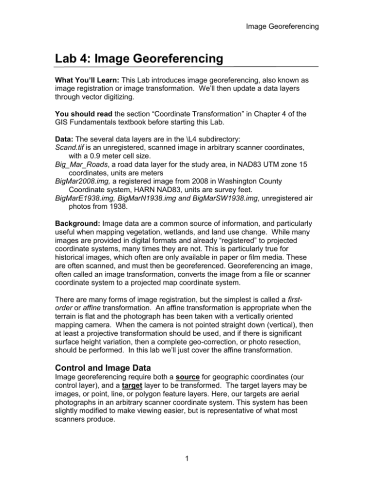
Image Georeferencing
Lab 4: Image Georeferencing
What You’ll Learn: This Lab introduces image georeferencing, also known as
image registration or image transformation. We’ll then update a data layers
through vector digitizing.
You should read the section “Coordinate Transformation” in Chapter 4 of the
GIS Fundamentals textbook before starting this Lab.
Data: The several data layers are in the \L4 subdirectory:
Scand.tif is an unregistered, scanned image in arbitrary scanner coordinates,
with a 0.9 meter cell size.
Big_Mar_Roads, a road data layer for the study area, in NAD83 UTM zone 15
coordinates, units are meters
BigMar2008.img, a registered image from 2008 in Washington County
Coordinate system, HARN NAD83, units are survey feet.
BigMarE1938.img, BigMarN1938.img and BigMarSW1938.img, unregistered air
photos from 1938.
Background: Image data are a common source of information, and particularly
useful when mapping vegetation, wetlands, and land use change. While many
images are provided in digital formats and already “registered” to projected
coordinate systems, many times they are not. This is particularly true for
historical images, which often are only available in paper or film media. These
are often scanned, and must then be georeferenced. Georeferencing an image,
often called an image transformation, converts the image from a file or scanner
coordinate system to a projected map coordinate system.
There are many forms of image registration, but the simplest is called a firstorder or affine transformation. An affine transformation is appropriate when the
terrain is flat and the photograph has been taken with a vertically oriented
mapping camera. When the camera is not pointed straight down (vertical), then
at least a projective transformation should be used, and if there is significant
surface height variation, then a complete geo-correction, or photo resection,
should be performed. In this lab we’ll just cover the affine transformation.
Control and Image Data
Image georeferencing require both a source for geographic coordinates (our
control layer), and a target layer to be transformed. The target layers may be
images, or point, line, or polygon feature layers. Here, our targets are aerial
photographs in an arbitrary scanner coordinate system. This system has been
slightly modified to make viewing easier, but is representative of what most
scanners produce.
1
Image Georeferencing
The control layer, in this case is a vector roads layer, is the source for your
control information. This control layer must be in the desired map coordinate
system. You will identify points in the control layer, and match them to
corresponding points in the target image. When you have enough points and are
satisfied with them, you create the transformed image (Video: Georeference).

Start QGIS.

Add Big_Mar_Roads.shp. This is our control layer, the one from which
we will get control locations.

Open the georeferencing tool under Raster – Georeferencer –
Georeferencer (see figure). This will open a Georeferencer window.

If you don’t see the Georeferencer under Raster, then you probably
have not activated the plugin. Do this via Plugins – Manage and install
plugins – All, then checking the Georeferencer-GDAL box

Add scand.jp2, our target layer, to the Georeferencer
window (NOT the main QGIS window), by clicking on the raster
icon in the upper left of the window.
2
Image Georeferencing
You should now have two windows open,
one for QGIS (see graphics at right), and
one labeled Georeferencer – scand1.tif
(below). Note how the menu along the top
bar changes when you click between
them. Also note that it says something like
“Transform: Not set” at the bottom of the
Georeferencer, and you may or may not
have a GCP (ground control point) window
showing.
Notice the icons on the Georeferencer
window to 1) Pan and zoom to control
point features, 2) add control points, and 3)
fit the georeferencing mode once you’ve added and edited the control points.
3
2
1
3
Image Georeferencing

If the GCP window is not displayed, activate the Georeferencer window,
then select View – Panels – GCP Table. This should display a blank
window, into which GCP will be placed when you digitize corresponding
points in the Georeferencer and main QGIS windows.
Georeferencing is done using by first selecting a point in the Georeferencer
window, using the Add Point Tool
:
then digitizing the same point in the QGIS window with the Edit Tool:
4
Image Georeferencing
Note that the selections should always proceed as:
1) mark a point in the Georeferencer window (the image), then
2) mark the corresponding point in the control layer displayed in the main
QGIS window (the roads in this case)
Now let’s digitize the control point pairs:

Use the zoom tools in the Georeferencer window to clearly display a
road intersection. Zoom in enough so that you may clearly see the width
of the road, and easily position the cursor in the middle of the road on the
image, e.g., the road intersection to the left of the eastern lobe of the lake
(graphic below):

Activate the Add Point Tool, and click on the center of the intersection
5
Image Georeferencing
This should display a window asking you to enter map coordinates:
If you had a list of coordinates, you could type them in the boxes. We don’t, and
will enter them from the map canvas.

Click on the green pencil/From map canvas button. The button should
turn blue (or some new color) to show it is active. The Georeferencer
window may “hide itself.” Don’t worry, it will come back in a bit.

Activate the edit
cursor, and zoom to
the corresponding
road intersection
found in the vector
roads data you’ve
displayed in the QGIS
map window (graphic
at right).

Make sure the edit
cursor is active, then
carefully place the
cursor the road
intersection in the
vector layer, and leftclick.
The Georeferencer image should come back, and the window labeled “Enter
map coordinates.”
Note there are now coordinates for the x and y values.

Click on the O.K. button to save the GCP. Note that the coordinate is
placed in the GCP table, and the Enter Map Coordinates window
disappears.
6
Image Georeferencing

Repeat this procedure, panning and zooming to a different road
intersection. First, click on the image (Georeferencer window), then on the
road layer version (QGIS window).
After you digitize your 4th GCP, fit the georeferencing model and examine the
resultant GCP Table. You fit the model with a

Click on the Start Georeferencing button
You’ll get a window saying you need to specify the transformation, dismiss it, and
fill out the Transformation settings as shown:

Set the transformation type to linear, the resampling can be nearest
neighbor or one of the averaging methods. Save the output to your
workspace, and set the Target SRS (coordinate system) and Target
resolution as shown.
7
Image Georeferencing
We know 1) the coordinate system specified is our intended output system, the
same one as the input roads layer from which we’re getting our coordinates. We
also know 2) that the image covers a small area and is effectively orthographic
(see textbook for definition), with the photo taken so as to be compatible with the
output coordinate system. We should always make sure these two conditions
hold.

Click O.K. on the Transformations Settings window once you’ve
entered the indicated values.
Note that it fits the model, georeferences the image to a new image, and writes
the residuals, or errors to the GCP table:
It also shows the model coeficients and the Mean Error or RMSE along the
bottom margin of the Georeferencer window (here about 20.1 meters).
The dX, dY, and overall residual give you some indication, although not the best
one, of how well the image has been georeferenced. You have too few control
links now, but this shows the process.

Add more points until you have at least ten control links. Note that as you
add each link, it re-fits the model and gives you a new set of residuals.
If you make a mistake, you can use the delete GCP tool to select and
delete a point. Alternately, you can turn it off in the table.
Remember to keep your points well distributed, try to have two points in each
quadrant of the image.

Now click again on the Start Georeferencing button. Notice that is
uses your previously entered settings, and fits a new model.

Add and remove control points until you have an RMSE you don’t think
you can improve on. Fit and save the image.

Write down your final Total RMSE value. You will later add this to you
final .pdf Map.

When you are done, Close the georeferencer window, save your points
table.
8
Image Georeferencing

Add your new registered image (BigMar2000.img).
Now digitize the current boundary of Big Marine Lake on your rectified image:
 Create a new polygon shapefile (Layer – New – Shapefile Layer), name it
Lake_2000, and specify the projection the same as the roads layer, NAD83
UTM zone 15.

Add this new empty lakes layer to your map

Start editing with the lakes layer as your target, and digitize the
boundary of Big Marine Lake, the large lake in the middle of the image, in
2000. Digitize at a scale of about 1:2500.
You may digitize the lake as one large polygon. Some prefer to digitize by
sections when creating large complex polygons. Do this by

Digitizing a portion as a polygon, then digitizing the next portion as a
closed polygon, making sure the polygons overlap completely at their
common edge.

Then select both polygons (Activate
tool, see figure at right, then drag a
rectangle that touches both)

Then use the merge tool on the polygons to create a single
polygon.

You are not required to “cut” out the islands inside the lake. It you wish to do
so, after you have completed the lake, make the lake layer semitransparent so you can see through it, and use the Add Ring tool
to cut out the island area from inside the lake.
You should now check the quality of your registration. You’ll do this by
comparing the image you just registered to a “test” image that is already in the
target coordinate system.
9
Image Georeferencing

First, close QGIS and then open
it again with a new canvas, and
add the image file
BigMar2008.img.
This is a bit lower resolution, and a bit
larger area than the image you used
before. Look at the coordinate
system, and units. This image is in
the Washington County Coordinate
System, HARN NAD83, in U.S. feet,
verifying this by comparing the
projection for the layer. Remember,
 to see the layer projection right
click on the image, select
properties, then General, and
expand the window for Coordinate reference system to see the parameters.
Compare the properties to those for the specification for Washington County in
the Minnesota County Coordinate Systems, found at:
http://www.dot.state.mn.us/surveying/toolstech/mapproj.html.

Load the image you just registered (named something like
BigMar2000.img) place it on top of the BigMar2008 image.
If the images don’t overlay properly, make sure QGIS is set to do “on the fly”
reprojection (if you don’t remember, see labs 1 & 2). If their still not aligned,
check the properties for the image you rectified (right click on the name in the
TOC, then Properties). Does it have the Coordinate system correctly listed as a
UTM NAD Zone 15N, in meters?). If not, you may have messed up the previous
projection, and so you should first try assigning the correct projection, and if that
doesn’t work re-do the digitizing).
 After you have the two images displayed correctly, click the top image on
and off, zooming to inspect the edge, to see how well your registration turned
out.
You may also make the top image semi-transparent, and compare the outline of
the lake to the image below it in the view.
To change the transparency,
 Right click on the top image, then Properties –Transparency, and set it to
50%
10
Image Georeferencing
Registering Historical Aerial Photographs
Now we will register three images from 1938 for Big Marine Lake. They are aerial
photographs taken during the dust bowl, a period of severe drought in the
Midwest, and perhaps the earliest photo of the area taken with a metric camera.
These images have been scanned, but not rectified to a coordinate system.

Open a new canvas, and add the image file BigMar2008.img.
 Open the Georeferencer, and add BigmarE1938.img to the window.
 Register this bigmarE1938.img image to the Washington County coordinate
system, U.S. Feet, using the BigMar2008.img as a source for control points.
Employ the techniques learned in the earlier parts of this lab.
Note that the 1938 image is not aligned north/south and doesn’t cover the entire
extent of the 2008 image, so you’ll have to be careful to pick corresponding
points.
Remember to:
Study the old image carefully FIRST. Many features have changed in the 72
years between images. Become familiar with the image.
Next select the control points, first in the target (unregistered 1938 image), and
then select the corresponding location in the control (color BigMar2008 image). A
figure on the following page shows suggested starting control points
Many features have changed over the years, so you may struggle to get enough
good points. Try to select 10 points, and select at least six. Make sure they are
as well distributed as possible.
You may get strange flips and distortions when fitting after just four points,
because the error of point selection dominates, and leads to transformation
equations that are wildly off the mark. If it does occur, it is best to delete the
target image (here the 1938 image) and start again.
 Use the process described in the previous section to create a set of GCPs,
and then rectify the image.
11
Image Georeferencing
Below are four suggested control points to help you start:
On saving the image, name it something like 1938East.img, so that you can
identify it later.
12
Image Georeferencing

Clear the canvas, and repeat the process for the Big_MarN1938,
registering as per the previous instructions.
See suggested starting control points below:
 Name the output 1938North.img
13
Image Georeferencing

Clear the QGIS date frame (or canvas), and add the Big_MarSW1938
image and register it following the previous instructions.
See suggested starting control points below:
14
Image Georeferencing
 Once all three images have been Georeferenced, open a new QGIS window
and load the base image and all three registered images. They should look
something like the figure below:
 Create a new polygon layer named Lake_1938. Import the coordinate
system from the BigMar2008.img.
 Digitize the lake boundary as it appeared in 1938.
The boundaries for a greatly reduced Big Marine Lake are apparent by the black
areas in the photos. The difference between the water and surrounding mud can
be subtle, you can use the map on the next page as a guide. Note that in some
photos the lake water is a bit lighter than others, due to sun/camera angles, so
look at all three photos in common areas to best identify the lake boundary. You
may want to reorder images when the overlap gets in the way of your digitizing,
or make adjacent images somewhat transparent to move from one image to
another.
15
Image Georeferencing
To Turn In:
Compose and export a Map as a .pdf, containing the transformed image
(BigMar2000) from the first part of the exercise, the roads, the lake boundary in
2000, the lake boundary in 1938, a scale bar, north arrow, title, and a legend.
See the example map at right.
Make sure you include the RMSE of your first transformation.
Remember, you are combining data from two different projections in this layout,
1) the image you rectified (UTM NAD83 zone 15N, meters), and 2) a Washington
County Coordinate System, HARN NAD83, in U.S. feet, so you have to make
sure the projections are properly assigned in each data layer, and select the
appropriate datum transformation (think about the two projections you are
combining when selecting among the datum transformation options).
16