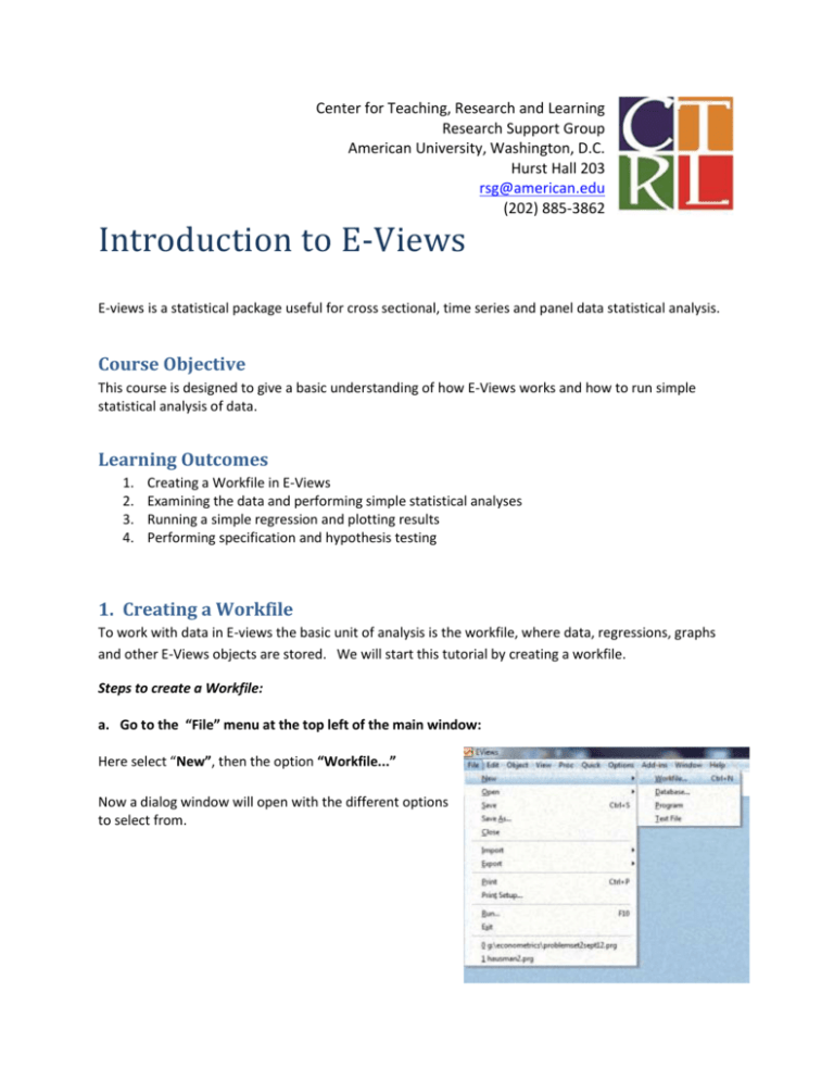
Center for Teaching, Research and Learning
Research Support Group
American University, Washington, D.C.
Hurst Hall 203
rsg@american.edu
(202) 885-3862
Introduction to E-Views
E-views is a statistical package useful for cross sectional, time series and panel data statistical analysis.
Course Objective
This course is designed to give a basic understanding of how E-Views works and how to run simple
statistical analysis of data.
Learning Outcomes
1.
2.
3.
4.
Creating a Workfile in E-Views
Examining the data and performing simple statistical analyses
Running a simple regression and plotting results
Performing specification and hypothesis testing
1. Creating a Workfile
To work with data in E-views the basic unit of analysis is the workfile, where data, regressions, graphs
and other E-Views objects are stored. We will start this tutorial by creating a workfile.
Steps to create a Workfile:
a. Go to the “File” menu at the top left of the main window:
Here select “New”, then the option “Workfile...”
Now a dialog window will open with the different options
to select from.
Introduction to E-Views CTRL
b. Indicate the type of Workfile you wish to create:
There are three data type options in E-Views: (i)
unstructured or undated data; (ii) dated/regular
frequency; and (iii) balanced panel.
For this exercise we will create a time series data set
for quarterly data, starting in the first quarter of 1952
and ending in the last quarter of 1996.
Therefore we should select in Workfile Structure Type
“Dated - regular frequency”. In Date Specification we
should select “Quarterly”. In start date type “1952.q1”
and in end date type “1996.4”.
Once the dialog box is filled, click the OK button. A workfile window will open.
c. Entering the data
There are two ways to enter data in an E-Views Workfile: manually and via importing from a
spreadsheet or text file.
Manually:
 In the workfile window, click on Objects/ New Object
 Specify type (for example: series) and
name the object (for example: GDP). Then
click OK.
2
Introduction to E-Views CTRL


In the Workfile Window double-click on
the variable name (GDP). A Window for
the GDP series will open. At the top of
this window Click on Edit and start
entering data.
Alternatively, one could “Copy and Paste”
the data from an Excel spreadsheet.
Importing Data from a spreadsheet:








First, verify that you have an open workfile to
receive the contents of the data imported and
that the workfile window is active.
For this exercise we will download the file
“Intro_Eviews.xls” from the CTRL Website at:
http://www.american.edu/provost/ctrl/training
guides.cfm
Store this file in your preferred location and
decompress it if necessary.
Select Proc /Import/Import from file…
Locate the data file “Intro_Eviews.xls” where
you store it for this exercise.
Step 1 of 3: E-views will open a window where it
will show a predefined range including all the
data in your Excel file.
Select custom range and start cell $B$1, this
way we do not copy the same time variable
indicating the quarters. (You can alternatively
leave the predefined range, click next and have
a variable for the time range).
Click “next”.
3
Introduction to E-Views CTRL




Step 2 of 3: A second window will be displayed
giving you the option to edit the name of the
variables and provide a description of them. For
this exercise provide the following sample
description for variable GDP: “Nominal Gross
Domestic Product for Country X”. You can also
provide descriptions for the other three variables
by clicking on them until they are shadowed:
o PR: Price level for Country X
o M1: Money supply for Country X
o RS: short-term interest rate for Country X
It is also important to indicate the units of your
data in the description (i.e., millions of local
currency) and your source, but for simplification
we obviate those details in this exercise.
Step 3 of 3: A third and final window will be
displayed where you should fill out the “start
date” of the data, in this case 1952q1.
Click “Finish”.
Now you will see all your series in the Workfile
window.
d. Saving the Workfile
 Click on the “Save” button in the workfile window.
Alternatively, select File/ Save As… or File/Save…
from the main menu.
 Select a location for the file and enter the name of
the file in the Save Window (i.e., we can save it
under the name “Example1”.
4
Introduction to E-Views CTRL
2. Examining the data and performing
simple statistical analyses and
transformations
a. Examining the contents of an individual series,
computing basic descriptive statistics and generating
charts.
 In the Workfile window double click on the
series that you wish to see, for example series
M1.
 Alternatively, select Quick/Show… in the main menu, enter m1, and click OK.
 Then, select View or Proc from the main menu.
 From this view you can now perform different
operations:
o Basic descriptive statistics
Click View/ select Descriptive Statistics &
Tests/ Histogram and Stats
You will now see a window with the histogram of the data
for M1 and a description of central tendency and
dispersion measures of the data.
5
Introduction to E-Views CTRL
o Charts
Select View/Graph..., and select Line & Symbol
from the list of graph types
b. Examining the contents of multiple series, computing basic descriptive statistics and generating
charts.
 We need to create a group for the series to
analyze.
In the Workfile window go to
Object/New Object and select “Group”. Then
click OK.
 A new window is displayed where you should
type the series that you want to include in the
group.
 The group is created, but is not saved until you
define a name for it. If you go to the tab options
at the upper side of the Group window you will
see the options “View”, “Proc”, “Object”, “Print”, “Name” and so on. Click on “Name” and a
new
window
will
appear giving you the
option to define a
name to identify the
group. The default
option is Group01,
which we will use for
this exercise.
 To examine your data
select
View/Descriptive
Statistics/Common
Sample and a window
with summary central
tendency and
dispersion measures will appear.
 To examine the covariance and correlation of the series select View/Covariance Analysis… A
window will appear in which you can select the options covariance and correlation.
6
Introduction to E-Views CTRL
o Charts
Select View/Graph..., and select Line & Symbol from the list of graph types. In the option
“Detail”, select the “single graph” if you want to see the four series in the same graph or
“multiple graph” if you want to see four different graphs.

Select View/Descriptive Stats/Individual Samples to display a table of descriptive statistics
computed for each of the series in the group
c. Transforming your data.
 A useful procedure that can be done with
E-Views is to transform your data and
generate variables, such as logarithms or
lagged variables.
 To generate logs: from the top of the
Workfile window select Genr and then
indicate a name for the transformed
variable that you want to create and the
transformation required. For example, if
you wish to create the logarithm of GDP
indicate that your new variable will be
called log_gdp and will be equal to
log(gdp). When estimating a regression you can simply
type log(gdp) without generating a new variable, as we
will see in point 3 below.
 To generate lags: from the top of the Workfile window
select Genr and then indicate a name for the transformed
variable that you want to create and the transformation
required. For example, if you wish to create the oneperiod lag of GDP indicate that your new variable will be
called gdp_1 and will be equal to gdp(-1), which refers to
the variable gdp lagged one period. When estimating a
regression you can simply type gdp(-1) without generating
a new variable, as we will see in point 3 below.
 To generate change of the series/first differences: similarly as before, but now we will define the
new variable as follows D(X)=X-X(-1), which indicates that the variable in difference is the
variable in the current time less the value in the previous period. If we generate this for gdp it
will be equivalent to d(gdp)=gdp-gdp(-1).
7
Introduction to E-Views CTRL
3. Running a regression
a. Estimating an equation

For this tutorial our example is the following
specification for a money supply model:
log(M1t) = b1 + b2log(GDPt)+b3RSt+b4Dlog(PRt)+
et
Where log(M1) is the logarithm of the money
supply, log(GDP) is the log of income, RS is the
short term interest rate, and Dlog(PR) is the log
first difference of the price level (the approximate
rate of inflation).

To estimate an equations go to the top menu of
the E-Views window, select Quick/Estimate
equation… and indicate the model you want to
estimate.

For this example we will indicate:
log(m1) c log(gdp) rs d(log(pr))
in the equation estimation window, where c
refers to the constant of the model and there is
no need to indicate the estimated beta
parameters.

In estimation settings we have different choices of estimators (LS, TSLS, GMM, ARCH, BINARY,
CENSORED, etc.). We will use the standard least squares -LS and set the appropriate sample
length (For example: 1952q1 1992q4). Then click OK.
b. Displaying actual & fitted values for the dependent variable, with residuals


Select View/Actual, Fitted, Residual/Table, and this will display a table containing the actual, the
fitted and the residual values of the estimation.
Select View/Actual, Fitted, Residual/Graph, and this will display a graph plot of the actual, the
fitted and the residual values of the estimation.
4. Specification and hypothesis tests
a. Performing hypothesis tests on the coefficients of the model
To test the hypothesis on the coefficients we can use the Wald test. As an example, we will test the
hypothesis that the coefficient on the price term is equal to 2.
 First, choose the coefficient of interest by selecting View/ Representations from the equation
toolbar
8
Introduction to E-Views CTRL

To test the restriction on C(4) you should select View/Coefficient Diagnostics/Wald–Coefficient
restrictions…, and enter in the dialog box the restriction c(4)=2
To test autocorrelation of order 1 we can use the Durbin-Watson statistic, which is shown at the
bottom of the Stats output of the regression. A value of approximately 2 will indicate there is no
evidence of autocorrelation of order 1. However, the Durbin-Watson test does not permit to test for
autocorrelation of higher order. The Durbin-Watson is approximately 0.16 for the estimated model,
indicating evidence of autocorrelation.
A more general autocorrelation test is the Breusch- Godfrey test for serial correlation in the residuals
 From the equation toolbar, select View/Residual Diagnostics/Serial Correlation LM Test…
 Then specify an order of serial correlation to test against. For example: entering 1 yields a test
against first-order serial correlation.
 Similarly to the Durbin-Watson test, the Breusch-Godfrey indicates there is evidence of serial
correlation of order 1. Therefore, we need to modify our original specification to take into
account the problem of serial correlation.
5. Modifying the equation specification
The new specification will be a transformation of the model in difference to correct the problem of
autocorrelation of the residuals. We will then indicate the following model in the estimation equation
window:
d(log(m1)) c d(log(gdp)) d(rs) d(log(pr))
Where d(log(M1)) is the difference of the logarithm of the money supply, d(log(GDP)) is the difference
of the log of income, d(RS) is the difference of the short term interest rate, and Dlog(PR) is the log first
difference of the price level (the approximate rate of inflation).
Click on Estimate
If we now test for autocorrelation, you can verify that there is no statistical evidence of autocorrelation
of the errors.
9