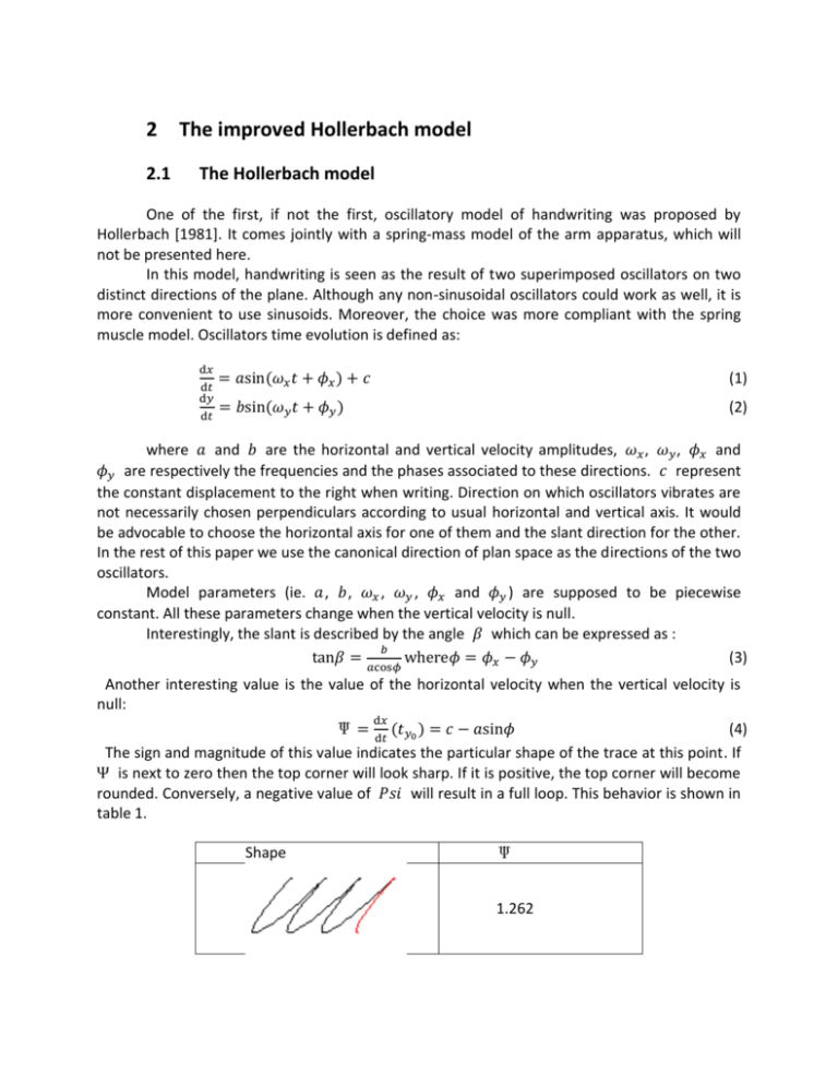
2
2.1
The improved Hollerbach model
The Hollerbach model
One of the first, if not the first, oscillatory model of handwriting was proposed by
Hollerbach [1981]. It comes jointly with a spring-mass model of the arm apparatus, which will
not be presented here.
In this model, handwriting is seen as the result of two superimposed oscillators on two
distinct directions of the plane. Although any non-sinusoidal oscillators could work as well, it is
more convenient to use sinusoids. Moreover, the choice was more compliant with the spring
muscle model. Oscillators time evolution is defined as:
d𝑥
d𝑡
d𝑦
d𝑡
= 𝑎sin(𝜔𝑥 𝑡 + 𝜙𝑥 ) + 𝑐
(1)
= 𝑏sin(𝜔𝑦 𝑡 + 𝜙𝑦 )
(2)
where 𝑎 and 𝑏 are the horizontal and vertical velocity amplitudes, 𝜔𝑥 , 𝜔𝑦 , 𝜙𝑥 and
𝜙𝑦 are respectively the frequencies and the phases associated to these directions. 𝑐 represent
the constant displacement to the right when writing. Direction on which oscillators vibrates are
not necessarily chosen perpendiculars according to usual horizontal and vertical axis. It would
be advocable to choose the horizontal axis for one of them and the slant direction for the other.
In the rest of this paper we use the canonical direction of plan space as the directions of the two
oscillators.
Model parameters (ie. 𝑎, 𝑏, 𝜔𝑥 , 𝜔𝑦 , 𝜙𝑥 and 𝜙𝑦 ) are supposed to be piecewise
constant. All these parameters change when the vertical velocity is null.
Interestingly, the slant is described by the angle 𝛽 which can be expressed as :
𝑏
tan𝛽 = 𝑎cos𝜙 where𝜙 = 𝜙𝑥 − 𝜙𝑦
(3)
Another interesting value is the value of the horizontal velocity when the vertical velocity is
null:
d𝑥
Ψ = d𝑡 (𝑡𝑦0 ) = 𝑐 − 𝑎sin𝜙
(4)
The sign and magnitude of this value indicates the particular shape of the trace at this point. If
Ψ is next to zero then the top corner will look sharp. If it is positive, the top corner will become
rounded. Conversely, a negative value of 𝑃𝑠𝑖 will result in a full loop. This behavior is shown in
table 1.
Shape
Ψ
1.262
-43.74
37.41
Table
1: The shape of the top corner of the trace depends on the sign and magnitude of Ψ.
2.2 Improving the oscillatory model
Hollerbach’s model does not address important questions:
1. Is there a way to quickly extract parameters, given a recorded trace ?
2. Is the ad-hoc 𝑐 parameter really necessary?
3. Parameters (𝑎, 𝑏, 𝜔𝑥 , 𝜔𝑦 , Φ𝑥 and Φ𝑦 ) are only allowed to change at
times of zero-crossing vertical velocity: is there any reason for this dissymmetry between x and
y axes ?
The main computational drawback of the Hollerbach model is the way we can get the
parameters from the trace: it is a non linear curve fitting problem. Usual optimizations methods
are costly; we will present an algorithm that is much more efficient. This efficiency is possible
because of our choice (that will be presented later) of the moments when parameters are
allowed to change. For a comparison between our method and usual optimization methods, see
[André,submitted].
The c parameter is of course representing the constant drift of the hand from left to
right when writing, but it seems a rather ad-hoc way for taking it into account. Moreover, it
imposes the X axis to be exactly aligned with the trace direction, and it introduces a
dissymmetry between X and Y. We will show that it can be simply omitted, and that the drift can
be accounted for by cumulating phase values between cycles.
About the dissymmetry between X and Y, it is true that the majority of shape changes
occur at Y velocity zero-values, which is visible in the fact that most loops and peaks are
directed upwards or downwards. However, an allograph such as “k” has clearly a parameter
change on the X velocity zero crossing near point a, which Hollerbach’s model cannot handle
properly.
2.3 The Improved Hollerbach Model
Our improved version of Hollerbach’s model is both simpler, symmetric and allows for a
fast parameters extraction algorithm. It is composed of a set of modelling equations, a model of
temporal changes and an algorithm of parameter extraction
1- Modelling equations. Oscillators time evolution is defined as:
d𝑥
d𝑡
d𝑦
d𝑡
= 𝑎𝑥 sin(𝜔𝑥 𝑡 + 𝜙𝑥 )
(3)
= 𝑎𝑦 sin(𝜔𝑦 𝑡 + 𝜙𝑦 )
(4)
2- Model of Parameters are constant by parts; they are allowed to change on X and Y
separately; X (resp. Y) changes only when X (resp. Y) velocity is null.
3- A trace is represented by :
a. A set of initial parameters values:
𝑎0 , 𝑏0 , 𝜔𝑥 0 , 𝜔𝑦 0 , Φ𝑥 0 and Φ𝑦 0
b. Two parameter series :
𝑆𝑥 = (𝑎𝑖, Φ𝑥 𝑖 )0≤𝑖≤𝑀
𝑆𝑦 = (𝑏𝑖, Φ𝑦 𝑖 )0≤𝑖≤𝑁
2.4 Extracting parameters from real traces
In this section we will present the algorithm used to retrieve parameters from a
recorded trace. In the remaining part of this paper, this algorithm will be referred to as the
direct method. Figure 1 shows the result of the direct method applied to a sentence. The
method is applied on each trace of the recorded sentence.
2.4.1 An interesting Mathematical result
Before moving on and describe our fast method to find the model parameters out of
recorded traces we need to demonstrate a proposition on harmonic functions. Consider the
following function:
𝑓: 𝑥 ↦ 𝑎sin(𝜔𝑥 + 𝜙)
(5)
where 𝑎, 𝜔 and 𝜙 are independant to 𝑥. First, let us calculate the mean and variance of 𝑓
between two successive zeros:
𝜋−𝜙
𝜔
𝜔 −𝜙
𝜔
𝜋−𝜙
𝜋
𝜔
𝜔 −𝜙
𝜔
𝑎2 (−8+𝜋2 )
𝑀=
𝜋
𝑉=
=
2𝑎
∫
𝑓(𝑥)𝑑𝑥 =
∫
(𝑓(𝑥) − 𝑀)2 𝑑𝑥
(6)
𝜋
(7)
2𝜋 2
Then, let us add the calculated mean and the square root of the calculated variance (ie.
the standard deviation) and divide the result by 𝑎:
𝑅 = 𝑀 + √𝑉
=2
𝑅
𝑎
=
√2√𝑎2 (−8+𝜋2 )
2𝜋
4+√2√−8+𝜋2 𝑠𝑔𝑛(𝑎)
𝑎
+
𝜋
(8)
(9)
2𝜋
Which if we give a numerical approximation leads to (if 𝑎 is positive):
𝑅
≈ 0.9443782250
𝑎
(10)
This result shows that the amplitude of a sinusoidal signal can be approximated by the
sum and standard deviation of this signal on a semi-period (zero to zero), independently of the
frequency and phase.
2.4.2
Evaluating trace parameters
Algorithm
Suppose the recorded trace is represented by a chronological finite list of time
stamped positions:
𝑆 = (𝑡𝑖 , 𝑥𝑖 , 𝑦𝑖 )0≤𝑖≤𝑁,𝑁∈ℕ∗,∀𝑖>0,𝑡𝑖 >𝑡𝑖−1
(11)
We apply the following steps on position components. Note that we present the steps for the
𝑥 component but it should be also applied to the y component.
Step 1
𝑥 = (𝑥𝑖 )0≤𝑖≤𝑁 is differentiated according to 𝑡 = (𝑡𝑖 )0≤𝑖≤𝑁 :
d𝑥
d𝑡
𝑥 −𝑥
= ( 𝑡𝑖 −𝑡 𝑖−1 )
𝑖
𝑖−1
0<𝑖≤𝑁
(12)
Step 2
Zeros are added to the beginning and to the end of the derivative signal. From a
theoretical point of view this could be contested: it is clear (for example if you look at the
pressure of the pen) that velocity is not always null when a writer begins or ends a trace ; but
we cannot infer this information from the time stamped positions only.
Step 3
We apply a zero-crossing algorithm on the derivative that we have previously low-pass
filtered (using a flat window of size 6). This prevents this algorithm to find clusters of zeros due
to acquisition irregularities or noise.
Step 4
Between two zeros, we said in section 2.2 that the parameters 𝑎, 𝜔𝑥 and 𝜙𝑥 were
constant. We now show that we can calculate these values easily. If 𝑡1 and 𝑡2 are the times of
two successive zero velocities, we have:
𝜔𝑥 (𝑡2 − 𝑡1 ) = 𝜋
𝜔𝑥 𝑡1 + 𝜙𝑥 = 0
(13)
(14)
From equation 13 we get 𝜔𝑥 and from equation 14 we get 𝜙𝑥 . This computation is
extremely simple and fast to perform; however it is very sensitive to errors during the zero
crossing algorithm. This point is developed further (5.1).
Step 5
The final step is to estimate the amplitude velocity 𝑎 (note that we still are between
two zero velocity times 𝑡1 and 𝑡2 ). Let us define 𝐴 as the part of the derivative signal
between 𝑡1 and 𝑡2 :
d𝑥
𝐴 = ( d𝑡 (𝑖)) between 𝑡 1 and 𝑡2
(15)
We approximate amplitude 𝑎 using result 3.1:
𝑎 = sign(𝐴)(mean(𝐴) + std(𝐴));
(16)
where 𝑠𝑖𝑔𝑛(𝐴) is the sign of the middle element of 𝐴 (notice that theorically, all elements
in 𝐴 are of the same sign).
2.4.3 Reconstructing the trace
From the previously calculated parameters a trace can be reconstructed. Knowing the initial
time, initial position and initial parameters 𝑎0 , 𝑏0 , 𝜔𝑥 0 , 𝜔𝑦 0 , Φ𝑥 0 and Φ𝑦 0 , we can calculate
the synthetized trace𝑆 ∗ = (𝑡𝑖 , 𝑥𝑖 ∗ , 𝑦𝑖 ∗ )0≤𝑖≤𝑁,𝑁∈ℕ∗,∀𝑖>0,𝑡𝑖 >𝑡𝑖−1 using only 𝑎, 𝑏, 𝜔𝑥 and 𝜔𝑦 .
Zero-crossing times, Φ𝑥 and Φ𝑦 , can be computed at reconstruction time, so there is no need
to store them.
Conversely, the time stamped positions in the trace can be reconstructed using:
- the initial time and position, and the initial parameter values 𝑎0 , 𝑏0 , 𝜔𝑥 0 , 𝜔𝑦 0 , Φ𝑥 0
and Φ𝑦 0
-
the extracted parameter values 𝑎𝑖 , 𝑏𝑖 , 𝜔𝑥 𝑖 , 𝜔𝑦 , Φ𝑥 𝑖 and Φ𝑦
𝑖
𝑖
The resulting function is a succession of half-periods of sinusoids whose parameters are given by
the series 𝑎𝑖 , 𝑏𝑖 , 𝜔𝑥 𝑖 , 𝜔𝑦 𝑖 , Φ𝑥 𝑖 and Φ𝑦 𝑖
Moreover, either the pair of Φ𝑥 𝑖 , Φ𝑦 𝑖 can be omitted in the series, because it can be inferred
from all other parameters
Finally, the complete reconstructed trace needs only 4 parameters per half period of writing.
Figure 1 shows an example of parameters extraction and of the reconstructed trace.