Ideal Answers to Chapter 7 (ANOVA) Questions
QUESTION 7.1a.
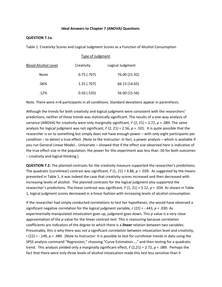
Table 1. Creativity Scores and Logical Judgment Scores as a Function of Alcohol Consumption
Type of Judgment
Blood Alcohol Level Creativity Logical Judgment
None 0.75 (.707) 76.00 (21.92)
.06%
.12%
1.25 (.707)
0.50 (.535)
66.13 (14.65)
56.00 (15.56)
Note. There were n=8 participants in all conditions. Standard deviations appear in parenthesis.
Although the trends for both creativity and logical judgment were consistent with the researchers’ predictions, neither of these trends was statistically significant. The results of a one-way analysis of variance (ANOVA) for creativity were only marginally significant, F (2, 21) = 2.72, p = .089. The same analysis for logical judgment was not significant, F (2, 21) = 2.56, p = .101. It is quite possible that the researcher is on to something but simply does not have enough power – with only eight participants per condition – to detect a true effect. [Note to the instructor: In fact, a power analysis – which is available if you run General Linear Model… Univariate – showed that if the effect size observed here is indicative of the true effect size in the population, the power for this experiment was less than .50 for both outcomes
– creativity and logical thinking.]
QUESTION 7.2. The planned contrasts for the creativity measure supported the researcher’s predictions.
The quadratic (curvilinear) contrast was significant, F (1, 21) = 4.86, p = .039. As suggested by the means presented in Table 1, it was indeed the case that creativity scores increased and then decreased with increasing levels of alcohol. The planned contrasts for the logical judgment also supported the researcher’s predictions. The linear contrast was significant, F (1, 21) = 5.12, p = .034. As shown in Table
1, logical judgment scores decreased in a linear fashion with increasing levels of alcohol consumption.
If the researcher had simply conducted correlations to test her hypotheses, she would have observed a significant negative correlation for the logical judgment variable, r (22) = -.443, p = .030. As experimentally manipulated intoxication goes up, judgment goes down. This p value is a very close approximation of the p value for the linear contrast test. This is reassuring because correlation coefficients are indicators of the degree to which there is a linear relation between two variables.
Presumably, this is why there was not a significant correlation between intoxication level and creativity,
r (22) = -.149, p = .489. [Note to Instructor: It is possible to test for curvilinear trends in data using the
SPSS analysis command “Regression,” choosing “Curve Estimation...,” and then testing for a quadratic trend. This analysis yielded only a marginally significant effect, F (2,21) = 2.72, p = .089. Perhaps the fact that there were only three levels of alcohol intoxication made this test less sensitive than it

otherwise might have been. Alternately, the fact that the inverted V pattern in these data wasn’t quite symmetrical simply meant that the effect doesn’t perfectly follow a quadratic pattern.]
QUESTION 7.3. In a horse race, a trifecta bet is a bet on the exact order of finish. Specifically, the bettor names which horse will finish first, second, and third. (A superfecta is the same thing but it involves six horses rather than three.) The bettor of a trifecta is only paid if his or her prediction matches perfectly the actual finishing order, but he or she is paid handsomely. In contrast, the bettor who placed a bet on each of the same three horses to “win, place, or show” would get paid if each of these three horses did place in the top three, but paid a lot less than a trifecta winner – because the second bettor didn’t make very precise predictions. In a sense, planned contrasts give researchers extra credit for more precise predictions. The researcher who conducts a planned contrast isn’t simply saying “some of these means
(horses) will be different (faster) than others.” Instead, he or she is predicting the exact pattern of results, loosely the equivalent of predicting the exact finishing order of multiple horses. Finally, just as it would be cheating to fill out a trifecta ticket and try to cash it in after a horse race had already finished, it would also be cheating to use planned contrasts that weren’t specified until after the results of a study were known.
QUESTION 7.4a. There was no main effect of self-esteem, F(1,16) = 0.00, p = 1.00. In fact, the F value was exactly zero because the average liking level for the confederate was identical for people low versus high in self-esteem. Both means were 5.5. There was also no main effect of feedback, F(1,16) = 0.00, p =
1.00. On average, people who got positive feedback did not like the confederate any more than those who got negative feedback. Again, both means were 5.5.
Although there were no main effects, there was a significant self-esteem x feedback interaction, F(1,16)
= 83.33, p < .001.
QUESTION 7.4b. Simple effects tests showed that the effect of feedback on liking was very different for people low versus high in self-esteem. Participants high in self-esteem esteem liked the confederate more when he gave them positive (M liking = 8.0) as opposed to negative (M liking = 3.0) feedback, t(8)
= -7.07, p < .001. Participants low in self-esteem esteem showed exactly the opposite preference. They liked the confederate more when he gave them negative (M liking = 8.0) as opposed to positive (M liking
= 3.0) feedback, t(8) = 5.98, p < .001.
QUESTION 7.4c. Self-enhancement theories predict that all people prefer positive feedback. These results do not support self-enhancement theories. Instead, they seem to support self-consistency theories such as Swann’s self-verification theory. This theory states that, because people rely on their self-views to predict and control their social worlds, people prefer other people who validate their existing self-views, even when these self-views happen to be negative.
QUESTION 7.4d. If we had failed to include self-esteem as a factor in this study, and had simply run a t- test to see if people preferred positive or negative feedback, we would have presumably obtained a null effect. This would have suggested that people are indifferent to social feedback. This is highly misleading. People do seem to have strong preferences. However, these preferences are very different for people low versus high in self-esteem.

QUESTION 7.5. Obviously, the answers to this question will vary enormously. Good answers will make it clear that an effect that occurs for one group of people, or under one manipulated set of experimental conditions, does not apply, or is actually reversed, for a different set of people, or under a different set of manipulated experimental conditions. The best answers will also make it clear that the pattern of means described flow directly from the writer’s chosen theory.
QUESTION 7.6. A 2 X 2 (Gender x Aggression Type) ANOVA yielded no main effect of aggression type, F <
1, p > .50. Surprisingly, however, the ANOVA did yield a main effect of gender, F (1,28) = 4.24. p = .049.
Averaging across the two types of aggression, girls (M = 7.25) were rated as more aggressive than were boys (M = 6.19). However, this main effect was qualified by a significant Gender x Aggression Type interaction, F (1,28) = 4.24, p = .049. Simple effects tests showed that there was no gender difference whatsoever for ratings of physical aggression, t (14) = 0.00, p = 1.00. The mean physical aggression rating for both boys and girls was 6.88. In contrast, there was a large gender difference for ratings of verbal aggressiveness, t (14) = -2.91, p = .010. Girls (M = 7.63) seem to have engaged in more verbal aggression than did boys (M = 5.50).
There are at least two reasons why it might be informative to conduct a follow-up study with adults. The lack of a gender difference on the measure of physical aggressiveness was highly unexpected, and it would be useful to explore this further. First, perhaps gender differences in physical aggressiveness only emerge, or become exaggerated, after puberty. Second, a drawback of having raters judge kids on verbal and physical aggressiveness is that raters may unknowingly hold boys and girls to different standards. For example, a rater who says that a 3-year old girl engaged in a highly physically aggressive act may (unknowingly) be applying different standards to boys and girls. Monica Biernat and colleagues have documented this kind of implicit gender bias numerous times in adults. As an obvious example, when people say that a woman is “tall,” what they usually mean is that she is taller than most women, not that she is 6’4”. Using an objective measure of both physical and verbal aggression would eliminate the need for human ratings and thus bypass any implicit gender biases that may have played a role in the lack of a gender effect on physical aggressiveness in this study of children. .
QUESTION 7.7. A 2 X 2 (Gender x Task Difficulty) ANOVA yielded a main effect of gender, F(1,28) = 7.39.
p = .011, as well as a main effect of task difficulty, F(1,28) = 8.73. p = .006. Both of these main effects were loosely consistent with predictions. Ignoring task difficulty, women paid themselves significantly less than men paid themselves, respective means were $5.81 and $7.25. Further, ignoring gender, people who got difficult anagrams paid themselves less than people who got easy anagrams, respective means were $7.31 and $5.75. In contrast to predictions, however, the gender x task difficulty interaction was not significant, F (1,28) = 2.36. p = .136. This result is somewhat ambiguous because the pattern of means suggests a very large gender difference for the hard anagrams and a much smaller gender difference for the easy anagrams (as predicted). It seems likely that if we could conduct some kind of planned contrasts for the total pattern of the four means, the results might confirm the predicted pattern. Nonetheless, in the absence of such a test, the safest, most traditional, interpretation is that the effect of gender is roughly equal for difficult and easy anagrams. Of course, the ultimate test of this idea would be replication. If the pattern observed here showed up consistently, a meta-analysis would surely yield a gender by task difficulty interaction.

QUESTION 7.8. The research does appear to have observed a three-way interaction. To begin, let’s focus solely on the individual priming words (such as I, me, and mine). For these words, the researcher clearly observed a 2-way Culture x Target Word Favorability interaction. In the individual primes condition,
American participants responded more quickly to the positive target words than to the negative target words. In contrast, Japanese participants showed exactly the opposite tendency. That is, after being exposed to individual primes, they responded more quickly to negative than to positive words. This is not only an interaction. It is apparently a cross-over interaction. When it comes to individual self-views,
Americans appear to have favorable self-associations whereas the Japanese have unfavorable selfassociations.
This tendency for Americans to be much more self-enhancing than the Japanese disappears, and even reverses somewhat, when we focus on group rather than individual primes. In the case of the group primes, there might be an interaction, too, but if so, it would be very roughly the opposite of the first interaction. Compared with American participants, Japanese participants showed an even more exaggerated tendency to respond more quickly to the favorable targets after having just been primed with group identity words (we, us, or ours).