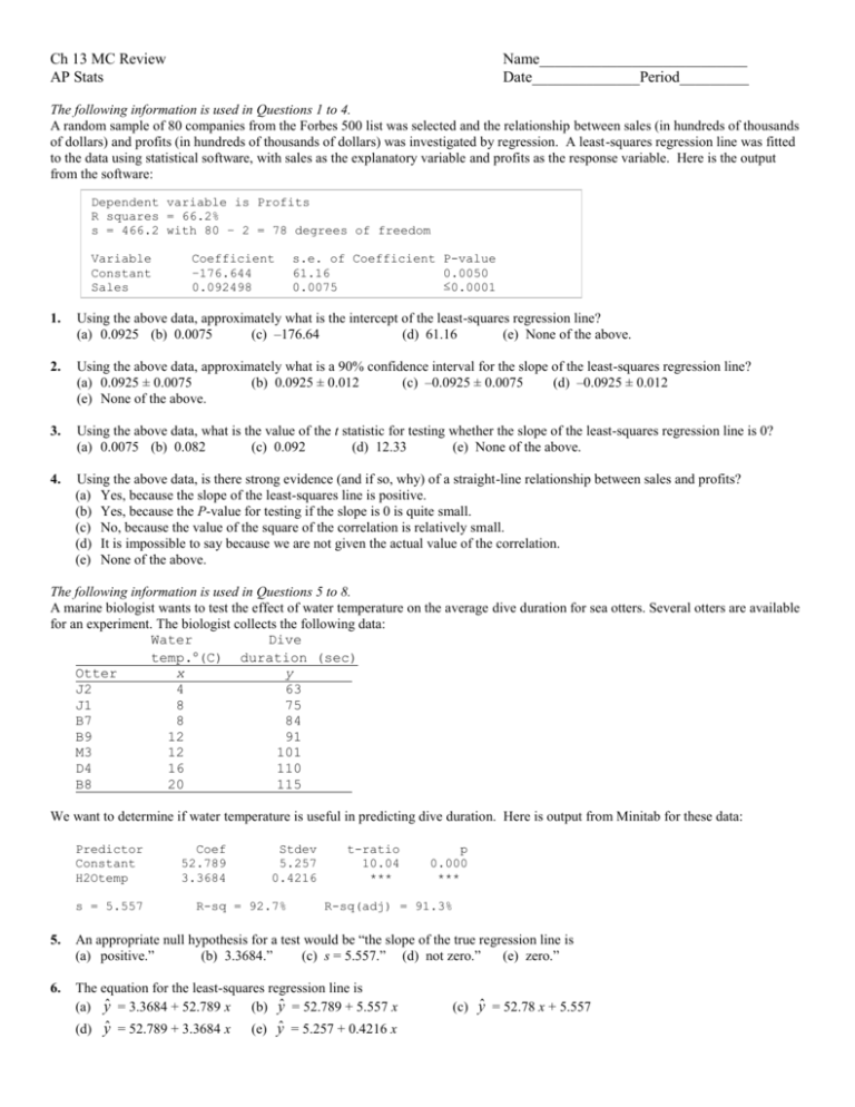
Ch 13 MC Review
AP Stats
Name___________________________
Date______________Period_________
The following information is used in Questions 1 to 4.
A random sample of 80 companies from the Forbes 500 list was selected and the relationship between sales (in hundreds of thousands
of dollars) and profits (in hundreds of thousands of dollars) was investigated by regression. A least-squares regression line was fitted
to the data using statistical software, with sales as the explanatory variable and profits as the response variable. Here is the output
from the software:
Dependent variable is Profits
R squares = 66.2%
s = 466.2 with 80 – 2 = 78 degrees of freedom
Variable
Constant
Sales
Coefficient
–176.644
0.092498
s.e. of Coefficient P-value
61.16
0.0050
0.0075
≤0.0001
1.
Using the above data, approximately what is the intercept of the least-squares regression line?
(a) 0.0925 (b) 0.0075
(c) –176.64
(d) 61.16
(e) None of the above.
2.
Using the above data, approximately what is a 90% confidence interval for the slope of the least-squares regression line?
(a) 0.0925 ± 0.0075
(b) 0.0925 ± 0.012
(c) –0.0925 ± 0.0075
(d) –0.0925 ± 0.012
(e) None of the above.
3.
Using the above data, what is the value of the t statistic for testing whether the slope of the least-squares regression line is 0?
(a) 0.0075 (b) 0.082
(c) 0.092
(d) 12.33
(e) None of the above.
4.
Using the above data, is there strong evidence (and if so, why) of a straight-line relationship between sales and profits?
(a) Yes, because the slope of the least-squares line is positive.
(b) Yes, because the P-value for testing if the slope is 0 is quite small.
(c) No, because the value of the square of the correlation is relatively small.
(d) It is impossible to say because we are not given the actual value of the correlation.
(e) None of the above.
The following information is used in Questions 5 to 8.
A marine biologist wants to test the effect of water temperature on the average dive duration for sea otters. Several otters are available
for an experiment. The biologist collects the following data:
Water
Dive
temp.(C) duration (sec)
Otter
x
y
J2
4
63
J1
8
75
B7
8
84
B9
12
91
M3
12
101
D4
16
110
B8
20
115
We want to determine if water temperature is useful in predicting dive duration. Here is output from Minitab for these data:
Predictor
Constant
H2Otemp
s = 5.557
Coef
52.789
3.3684
Stdev
5.257
0.4216
R-sq = 92.7%
t-ratio
10.04
***
p
0.000
***
R-sq(adj) = 91.3%
5.
An appropriate null hypothesis for a test would be “the slope of the true regression line is
(a) positive.”
(b) 3.3684.”
(c) s = 5.557.” (d) not zero.”
(e) zero.”
6.
The equation for the least-squares regression line is
(a) ŷ = 3.3684 + 52.789 x (b) ŷ = 52.789 + 5.557 x
(d) ŷ = 52.789 + 3.3684 x
(e) ŷ = 5.257 + 0.4216 x
(c) ŷ = 52.78 x + 5.557
7.
The t statistic for testing H0 has been left out. From the output, the t-statistic has the value
(a) 7.99.
(b) 10.04.
(c) 0.124.
(d) 0.927.
(e) 15.67.
8.
The P-value is
(a) less than 0.001.
(d) between 0.05 and 0.10.
(b) between 0.001 and 0.01.
(e) greater than 0.10.
(c) between 0.01 and 0.05.
Questions 9 to 17 are based on the following information.
Florida reappraises real estate every year, so the county appraiser’s Web site lists the current “fair market value” of each piece of
property. Property usually sells for somewhat more than the appraised market value. Here are the appraised market values and actual
selling prices (in thousands of dollars) of condominium units sold in a beachfront building over a 19-month period:
Selling
price
850
900
625
1075
890
810
650
845
Appraised
value
758.0
812.7
504.0
956.7
747.9
717.7
576.6
648.3
Selling
price
790
700
715
825
675
1050
1325
845
Month
0
1
2
2
8
8
9
12
Appraised
value
605.9
483.8
585.8
707.6
493.9
802.6
1031.8
586.7
Month
13
14
14
14
17
17
18
19
Here is part of the Minitab output for regressing selling price on appraised value.
Predictor
Constant
appraisal
S = 69.7299
Coef
127.27
1.0466
SE Coef
79.49
0.1126
R-Sq = 86.1%
T
1.60
9.29
P
0.132
0.000
R-Sq(adj) = 85.1%
Predicted Values for New Observations
New
Obs
1
9.
Fit
967.3
SE Fit
21.6
95% CI
(920.9, 1013.7)
95% PI
(810.7, 1123.9)
The equation of the least-squares regression line for predicting selling price from appraised value is
(a) price = 79.49 + 0.1126  appraised value.
(b) price = 127.27 + 1.0466  appraised value.
(c) price = 1.0466 + 127.27  appraised value.
(d) price = 127.27 + 69.7299  appraised value.
(e) price = 79.49 + 1.0466  appraised value.
10. What is the correlation between selling price and appraised value?
(a) 0.1126 (b) 0.861 (c) 0.928
(d) 0.851 (e) 0.922
11. The slope  of the population regression line describes
(a) the exact increase in the selling price of an individual unit when its appraised value increases by $1000.
(b) the average increase in selling price in a population of units when appraised value increases by $1000.
(c) the average selling price in a population of units when a unit’s appraised value is 0.
(d) the predicted increase in appraised value when the selling price increases by $1000.
(e) the exact increase in appraised value when the selling price increases by $1000.
12. Is there significant evidence that selling price increases as appraised value increases? To answer this question, test the hypotheses
(a) H0:  = 0 versus Ha:  > 0.
(b) H0:  = 0 versus Ha:  ≠ 0.
(c) H0:  = 0 versus Ha:  > 0.
(d) H0:  = 0 versus Ha:  < 0.
(e) H0:  > 0 versus Ha:  = 0.
13. The P-value for this test is
(a) less than 0.001.
(b) between 0.001 and 0.005.
(c) between 0.005 and 0.05.
(d) between 0.05 and 0.10.
(e) greater than 0.10.
14. The regression standard error for these data is
(a) 0.1126.
(b) 69.7299.
(c) 79.49.
(d) 21.6.
(e) 967.3.
15. Confidence intervals and tests for these data use the t distribution with degrees of freedom
(a) 14.
(b) 15.
(c) 16.
(d) 30.
(e) 17.
16. A valid conclusion to our analyses is that
(a) there is insufficient evidence to conclude that the slope of the true regression line is not zero.
(b) there is insufficient evidence to conclude that the slope of the true regression line for these 19 condominium units is $10,466.
(c) there is strong evidence to conclude that selling price increases as the appraised value increases.
(d) there is weak evidence that  is positive.
(e) there is evidence to conclude that the slope of the true regression line is significantly greater than zero.
17. A 95% confidence interval for the population slope  is
(a) $1.0466 ± 0.2415.
(b) $1.0466 ± 149.5706.
(c) $1.0466 ± 0.2387.
(d) 967.3 ± 46.4.
(e) 967.3 ± 156.6.
ANSWERS
1. C
8. A
15. E
2. B
9. B
16. C
3. D
10. C
17. C
4. B
11. B
5. E
12. A
6. D
13. A
7. A
14. B