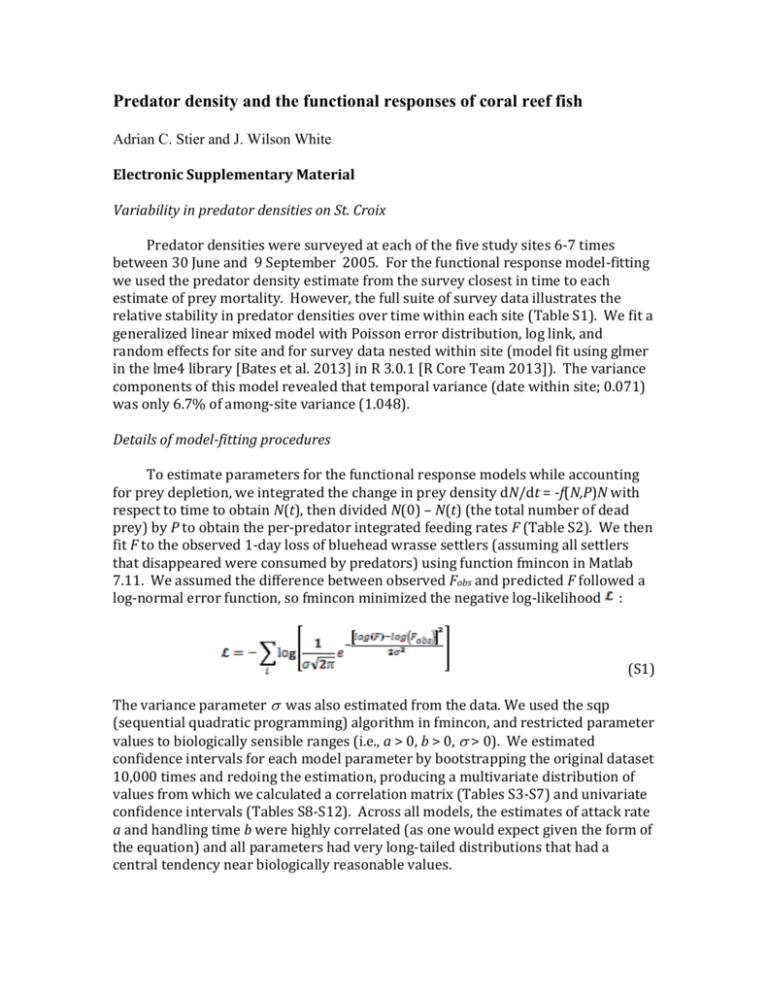
Predator density and the functional responses of coral reef fish
Adrian C. Stier and J. Wilson White
Electronic Supplementary Material
Variability in predator densities on St. Croix
Predator densities were surveyed at each of the five study sites 6-7 times
between 30 June and 9 September 2005. For the functional response model-fitting
we used the predator density estimate from the survey closest in time to each
estimate of prey mortality. However, the full suite of survey data illustrates the
relative stability in predator densities over time within each site (Table S1). We fit a
generalized linear mixed model with Poisson error distribution, log link, and
random effects for site and for survey data nested within site (model fit using glmer
in the lme4 library [Bates et al. 2013] in R 3.0.1 [R Core Team 2013]). The variance
components of this model revealed that temporal variance (date within site; 0.071)
was only 6.7% of among-site variance (1.048).
Details of model-fitting procedures
To estimate parameters for the functional response models while accounting
for prey depletion, we integrated the change in prey density dN/dt = -f(N,P)N with
respect to time to obtain N(t), then divided N(0) – N(t) (the total number of dead
prey) by P to obtain the per-predator integrated feeding rates F (Table S2). We then
fit F to the observed 1-day loss of bluehead wrasse settlers (assuming all settlers
that disappeared were consumed by predators) using function fmincon in Matlab
7.11. We assumed the difference between observed Fobs and predicted F followed a
log-normal error function, so fmincon minimized the negative log-likelihood :
(S1)
The variance parameter  was also estimated from the data. We used the sqp
(sequential quadratic programming) algorithm in fmincon, and restricted parameter
values to biologically sensible ranges (i.e., a > 0, b > 0, > 0). We estimated
confidence intervals for each model parameter by bootstrapping the original dataset
10,000 times and redoing the estimation, producing a multivariate distribution of
values from which we calculated a correlation matrix (Tables S3-S7) and univariate
confidence intervals (Tables S8-S12). Across all models, the estimates of attack rate
a and handling time b were highly correlated (as one would expect given the form of
the equation) and all parameters had very long-tailed distributions that had a
central tendency near biologically reasonable values.
One difficulty in estimation was that Eq. S1 cannot be evaluated if Fobs is equal
to zero (no observed deaths) or to (which results when predator density = 0).
Rather than exclude those observations, we assumed that both mortality and
predator density were observed with some error, so it was unlikely that either value
was exactly zero. Therefore for those cases we set Fobs to be equal to the minimum
non-zero or maximum finite values observed in the dataset. The ordering of results
(i.e., which model was most parsimonious) was robust to alternative corrections we
applied, such as making the minimum value 10% or 1% of the minimum observed
non-zero value, so we are confident that applying this correction did not produce
arbitrary conclusions.
Table S1. Summary of predator survey data on St. Croix reefs in 2005.
Site
BB
CB
NS
JB
WC
n
(number of surveys)
7
7
7
6
7
Mean coney grouper density
(number per 150 m2)
3.4286
2.8674
6.1198
0.5000
0.4858
Table S2. Time-integrated solution for each functional response model
Model
Formula
H2
BD
CM
HV
RD
Note:  denotes the Wright omega function
Table S3. Correlation matrix for H2 model parameters
a
b

a
1
0.9256
210-16
b
1
-210-14
1

Table S4. Correlation matrix for BD model parameters
a
b

a
1
0.9904
0.9620
-0.0308
b
1
0.9232
-0.0144
c
1
-0.0367
1

Table S5. Correlation matrix for CM model parameters
a
b

a
1
0.9896
0.1756
-0.0153
Standard
error
0.3770
0.3527
0.3527
0.4072
0.3683
b
c

1
0.1800
1
-0.0130
-0.0426
1
Table S6. Correlation matrix for HV model parameters
a
b
m

a
1
0.8059
0.6678
0.1051
b
1
0.4226
0.1519
m
1
0.2501
1

Table S7. Correlation matrix for RD model parameters
a
b

a
1
0.9953
-0.0053
b
1
-0.0023
1

Table S8. Confidence intervals (95%) for H2 model parameters
Parameter
lower
median
upper
a
0.1816
0.3391
17.1913
b
0.0242
14.7720
1.010-10
1.6871
1.6871
1.6871

Table S9. Confidence intervals (95%) for BD model parameters
Parameter
lower
median
upper
a
0.1908
0.7411 434.1583
b
0.1880 197.2059
1.010-10
-10
c
0.5587
0.8424
1.010
0.5140
0.8424
1.0588

Table S10. Confidence intervals (95%) for CM model parameters
Parameter
lower
median
upper
a
0.1780
1.4853 648.6314
-10
b
0.4090 261.8480
1.010
c
-0.0921
0.6584
2.7845
0.5166
0.8194
1.0665

Table S11. Confidence intervals (95%) for HV model parameters
Parameter
lower
median
upper
a
0.1654
1.4601
11.9923
b
0.0102
0.9092
8.7194
m
0.1417
0.8899
2.1249
0.5389
0.8258
1.2121

Table S12. Confidence intervals (95%) for RD model parameters
Parameter
lower
median
upper
a
0.4508
1.1501
9.6793
b
0.1858
0.5478
10.5260
0.5318
0.8724
1.1095
