BIOINF 2118 01-Introduction to Probability
p.1 of 6
Probability and Statistics
Probability:
Process
Data
“Given a process or mechanism,
after many repetitions what kinds of outcomes (data) can we expect?”
Statistics:
Data
Process
“Given some data,
what can we say about the process or mechanism that gave rise to the data?”
Example: Diagnostic testing
A patient arrives in the clinic. The doctor suspects that the patient suffers a particular illness.
The true state, “healthy” or “sick”, is unknown; therefore the doctor orders a diagnostic test.
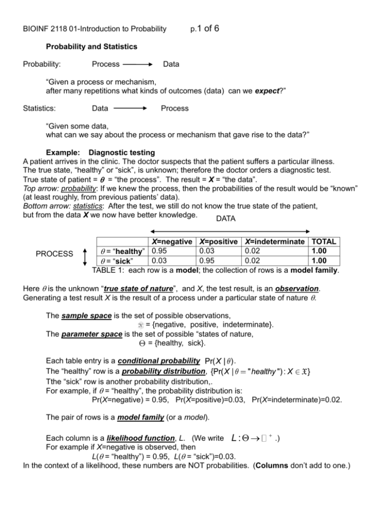
True state of patient =  = “the process”. The result = X = “the data”.
Top arrow: probability: If we knew the process, then the probabilities of the result would be “known”
(at least roughly, from previous patients’ data).
Bottom arrow: statistics: After the test, we still do not know the true state of the patient,
but from the data X we now have better knowledge.
DATA
PROCESS
X=negative X=positive X=indeterminate TOTAL
0.03
0.02
1.00
 = “healthy” 0.95
0.03
0.95
0.02
1.00
 = “sick”
TABLE 1: each row is a model; the collection of rows is a model family.
Here  is the unknown “true state of nature”, and X, the test result, is an observation.
Generating a test result X is the result of a process under a particular state of nature .
The sample space is the set of possible observations,
X = {negative, positive, indeterminate}.
The parameter space is the set of possible “states of nature,
= {healthy, sick}.
Each table entry is a conditional probability
.
The “healthy” row is a probability distribution,
Tthe “sick” row is another probability distribution,.
For example, if  = “healthy”, the probability distribution is:
Pr(X=negative) = 0.95, Pr(X=positive)=0.03, Pr(X=indeterminate)=0.02.
The pair of rows is a model family (or a model).
+
Each column is a likelihood function, L. (We write L : Q ®
.)
For example if X=negative is observed, then
L( = “healthy”) = 0.95, L( = “sick”)=0.03.
In the context of a likelihood, these numbers are NOT probabilities. (Columns don’t add to one.)
BIOINF 2118 01-Introduction to Probability
p.2 of 6
Now suppose that the prevalence of the disease is 10%. Prevalence = Pr( = “sick”).
The following table is the joint distribution of  and X.
X=negative
X=positive
X=indeterminate
0.855
0.027
0.018
0.003
0.095
0.002
0.858
0.122
0.020
TABLE 2: joint probabilities for each combination
 = “healthy”
 = “sick”
TOTAL
TOTAL
0.90
0.10
1.00
Interpretations of Probability
•Frequency interpretation:
“
” means:
“If I do the test repeatedly on a large number of sick patients,
then in the long run roughly 95% of the test results will equal positive.
•Subjective (Bayesian) interpretation- before data is observed:
, which means:
“Given what I know now,
my current belief is that there’s a 10% chance that this patient is sick.”
Connection with decision-making:
This belief sometimes represents a willingness to gamble that the patient is sick,
if the payoff is above the ratio 9-to-1 (0.9/0.1), but not if it’s below 9-to-1.
•Subjective (Bayesian) interpretation- after data is observed:
X=negative (1) X=positive (2) X=indeterminate (3)
0.221
0.9
 = “healthy” 0.9965
0.0035
0.779
0.1
 = “sick”
TOTAL
1.0000
1.000
1.0
TABLE 3: conditional probabilities, given X
,which means:
“Given what I knew before, plus what I know now (the data),
my current belief is that there’s a 77.9% chance that this patient is sick.”
Table 3 combines the two types of probability: belief and frequency.
Now the gambling odds are 0.779/(1-0.779) = 3.52.
BIOINF 2118 01-Introduction to Probability
p.3 of 6
NOTATION and TERMINOLOGY
“Statistics” is assessing whether the patient is healthy or sick, after observing X.
We saw this above, in the form of the posterior probability, 0.779.
When the prevalence is not known, we have to use the frequency interpretation of probability, using
the models in TABLE 1. A great tool is the likelihood ratio, LR:
.
LR(X=1) = 0.03/0.95 ~ 1/32, LR(X=2) =0.95/0.03 ~ 32, LR(X=3) = 1.
The LR compares two explanations for the observation.
Here we see that the observation X=negative lowers the probability of “sick”, and X=positive
raises it. Observing X=indeterminate does not provide any information, as reflected in LR=1.
For each value of X, we can see in what way the value of the probability changes, but we cannot say
what the final probability is because we do not know the initial probability.
Experiments
•An experiment is any process in which the outcome is uncertain.
•Examples: Rolling a die, conducting a clinical trial, conducting a survey, getting married,….
•The sample space X is the set of possible outcomes.
•Example: For our diagnostic test, X = {1, 2, 3}. For rolling a die, X = {1, 2, 3, 4, 5, 6}.
Sets and Subsets
•A sample space X is a set.
•An outcome is an element of the sample space,
.
•An event is a subset of the sample space. For example,
is the event of rolling an
even number with a die.
•An event A implies another event B if every outcome in A also belongs to B. This relation is
denoted
, “A is a subset of B”.
•A parameter space
is a set.
•A hypothesis is a subset
.
Empty, Finite and Infinite Sets
•The empty set contains no outcomes. It is denoted by . For all events A,
•Sets may be finite or infinite.
is finite.
•Infinite sets may be countably infinite or uncountably infinite.
X =[0,1] is uncountable.
is countable (but infinite).
.
BIOINF 2118 01-Introduction to Probability
Union, Intersection, Complement
Concept
union (either/or)
intersection (both)
complement (not)
Ac
or { }
empty set, or null set
set product
X
Subset
element of
p.4 of 6
symbol
Disjoint Events
•A and B are disjoint if and only if
.
.
•Events
are disjoint or mutually exclusive if, for every
R function or value
union( )
intersect( )
setdiff( )
NULL, character(0)
expand.grid( )
all(is.element( ))
is.element( )
.
p.5 of 6
BIOINF 2118 01-Introduction to Probability
Some formal definitions:
A probability space is a sample space X, together with a mapping Pr from events in a sample space
to [0,1] (in mathematical notation, Pr: 2X  [0,1]) that satisfy three axioms:
Axiom 1: For every event A
,
.
(To be technically correct: there may be very esoteric sets which cannot be assigned a probability.)
Axiom 2: Pr(X) = 1.
Axiom 3: For every “countable” sequence of disjoint events
,
Some probability theorems:
Given a parameter space
and a sample space X,
a model family indexed by
is a set of probability distributions
.
When X is observed, the likelihood function is the function
defined by
.
(Later, we’ll modify this slightly for “continuous distributions”.)
The likelihood function:
= the parameter space
The probability model:
X
= the sample space
BIOINF 2118 01-Introduction to Probability
p.6 of 6
HOMEWORK #1, due date = class #3.
Exercise 1.1
 STUDY CAREFULLY ALL NOTATION AND DEFINITIONS. 
Make a list of the terms introduced in Class #01 document, and their definitions.
Make a list of any notations in this document that were unfamiliar;
indicate whether the meaning is still unclear to you.
Exercise 1.2
Go to www.r-project.org , download and install R.
Go to www.rstudio.org , download and install RStudio. It works on all the platforms.
Here are some resources to help you learn R:
http://cran.r-project.org/doc/manuals/R-intro.html
Read sections 1,2,5,9,10.
Do the sample session in subsection 1.6.
Save/print out your session and turn it in (by e-mail).
Exercise 1.3
Read Appendix B in Shahbaba’s book.
Don’t worry about the details, just get a sense of the concepts.