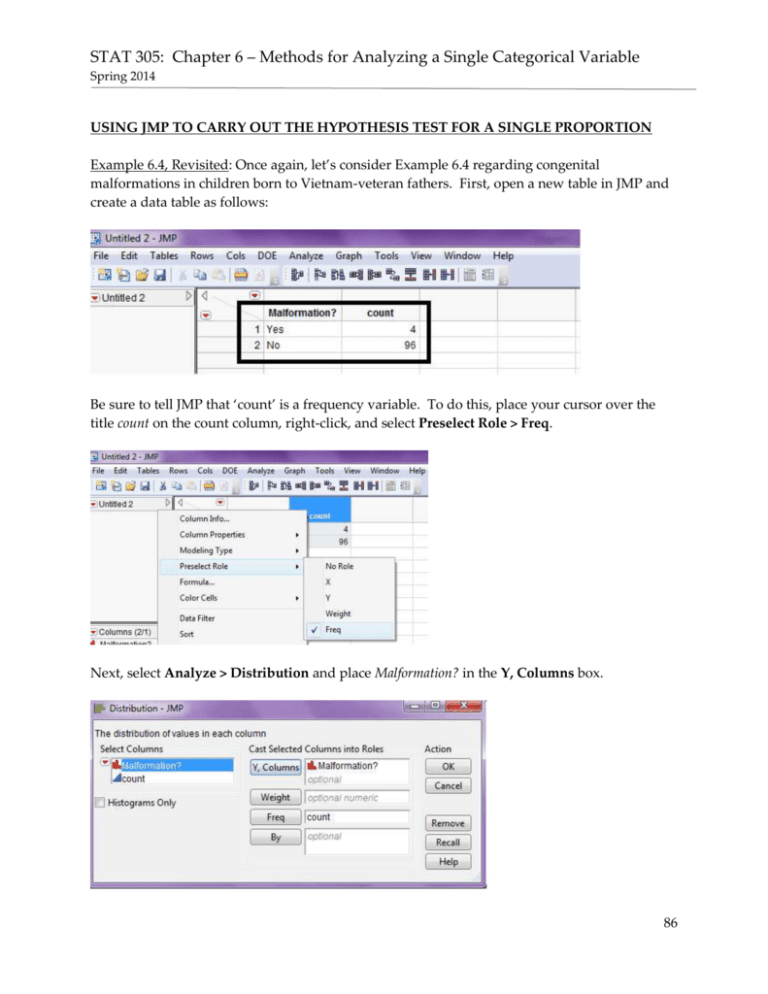
STAT 305: Chapter 6 – Methods for Analyzing a Single Categorical Variable
Spring 2014
USING JMP TO CARRY OUT THE HYPOTHESIS TEST FOR A SINGLE PROPORTION
Example 6.4, Revisited: Once again, let’s consider Example 6.4 regarding congenital
malformations in children born to Vietnam-veteran fathers. First, open a new table in JMP and
create a data table as follows:
Be sure to tell JMP that ‘count’ is a frequency variable. To do this, place your cursor over the
title count on the count column, right-click, and select Preselect Role > Freq.
Next, select Analyze > Distribution and place Malformation? in the Y, Columns box.
86
STAT 305: Chapter 6 – Methods for Analyzing a Single Categorical Variable
Spring 2014
On the resulting output, click on the red drop-down arrow next to Malformation? and choose
Test Probabilities.
Next, enter the hypothesized probabilities into JMP as follows. Note that you must tell JMP that
this is an upper-tailed test.
Finally, click Done, and JMP returns the p-value for the upper-tailed exact binomial test:
87
STAT 305: Chapter 6 – Methods for Analyzing a Single Categorical Variable
Spring 2014
Example 6.6, Revisited: Reconsider Example 6.6 regarding female ecology majors. Create a data
table as follows:
Once again, place your cursor over the count column and select Preselect Role > Frequency.
Then, select Analyze > Distribution and place Gender in the Y, Columns box. Click OK, and
you should see the following:
Click on the red drop-down arrow next to Gender and select Test Probabilities. Enter the
hypothesized probabilities as follows:
88
STAT 305: Chapter 6 – Methods for Analyzing a Single Categorical Variable
Spring 2014
Note that we once again used an upper-tailed test in JMP, even though earlier in the notes we
stated that Example 6.6 was an example of a lower-tailed test. Why is this? Before, we were
focusing on the proportion of females which would be less than expected if females were underrepresented. However, JMP is focusing on the proportion of males, which would be greater than
expected if females were under-represented. Click done, and JMP returns the following:
Example 6.7, Revisited: Reconsider Example 6.7 regarding ear infections in breast-fed vs. bottlefed babies.
Go through steps similar to those of the following examples until you obtain the following:
89
STAT 305: Chapter 6 – Methods for Analyzing a Single Categorical Variable
Spring 2014
The output is as follows:
Note that this p-value does not match our p-value from earlier (although it is very close). This
is because for two-sided tests, JMP does not use the binomial distribution to find p-values.
Instead, it uses the chi-square distribution (which will be discussed later in the semester).
CONFIDENCE INTERVALS
Unlike hypothesis testing, this procedure does NOT require any hypotheses concerning our
population parameter of interest. Instead, this interval will give us a range of likely values for
this parameter.
Comments:
1. A confidence interval allows us to estimate the population parameter of interest (note
that the hypothesis test does NOT allow us to do this). Therefore, when available, a
confidence interval should always accompany the hypothesis test.
2. Several methods exist for constructing a confidence interval for a binomial proportion;
however, we will focus on only the “score method” which is used by JMP. This method
is carried out for Example 6.6 (females in ecology) as follows:
The Formula for the Score Confidence Interval:

n = sample size =

π̂ = sample proportion =

z = appropriate percentile from the standard normal distribution
90
STAT 305: Chapter 6 – Methods for Analyzing a Single Categorical Variable
Spring 2014
Confidence Level
z
90%
1.645
95%
1.96
99%
2.58
Plug these values into the following equation:
2nπ̂  z  
2n  z 
2

z z 2  4nπ̂(1  π̂)
2

2 n  z2

  JMP approach
An easier, though slightly less accurate version of a 100(1-CI for 
𝜋̂ ± 𝑧√
̂ (1−𝜋
̂)
𝜋
𝑛
 By hand approach
Note that this gives us a range of values that is close to the “middle 95%” of the binomial
distribution with n = 41 and p = 20/41 = .4878.
91
STAT 305: Chapter 6 – Methods for Analyzing a Single Categorical Variable
Spring 2014
Calculating the Score Confidence Interval in JMP:
To find the 95% confidence interval for the population proportion of females majoring in
ecology, select the red drop-down arrow next to the variable name and choose Confidence
Interval > .95.
JMP then returns the confidence interval:
Interpretation of this Confidence Interval:
92
STAT 305: Chapter 6 – Methods for Analyzing a Single Categorical Variable
Spring 2014
Margin of Error: The margin-of-error is defined as the distance between the center of the
confidence interval and either endpoint. For this problem, we have
Upper Endpoint – Center of Interval =
So, the margin of error for this problem is:
Questions:
1. What happens to the margin of error when the confidence level decreases? For example,
what will happen if we use a 90% confidence level instead of 95%?
2. What will happen to the margin of error and the c onfidence interval if we increase the
level of confidence?
Example 6.8: In 2005, marine biologists of James Cook University in Queensland, Australia,
carried out a study to investigate the proportion of fish that return to their birthplace. They
captured all adult female clown fish from a coral reef near Papua New Guinea’s Kimbe Island
and then injected them with an isotope that would be passed on to the female’s developing
eggs. This isotope was naturally incorporated into the bones of the offspring. Since the
particular isotope used was very rare in nature, its presence in the offspring was a very effective
tag.
93
STAT 305: Chapter 6 – Methods for Analyzing a Single Categorical Variable
Spring 2014
The offspring then spent a few weeks in the open ocean, and
the researchers returned to the same reef and captured 15
clown fish that were settled there. Nine of the 15 fish contained
the barium isotope; that is, of the 15 sampled fish that had
settled at the reef, 9 had been spawned there.
Source: Science 4 May 2007: Vol. 316 no. 5825, pp. 742-744. A link to a press release regarding
this article is given here.
Research Question: Do the data provide evidence that the majority of the juvenile clown fish
settled at the reef had been spawned there?
Questions:
1. What is the population of interest?
2. What is the variable of interest (i.e., our response variable)?
3. What is the parameter of interest? The sample statistic?
Carry out a hypothesis test to address this research question:
Step 1:
Set up the null and alternative hypotheses.
Ho: The fish that had been spawned at the reef do not make up the
majority of the clown fish population.
Ha: The majority of clown fish settled at the reef were spawned there.
Step 2:
Find the Critical Value/Critical Region or p-value.
We can use the binomial distribution with n = 15 and π = .5.
94
STAT 305: Chapter 6 – Methods for Analyzing a Single Categorical Variable
Spring 2014
We can also use JMP:
Step 3:
Write a conclusion regarding the research question.
95
STAT 305: Chapter 6 – Methods for Analyzing a Single Categorical Variable
Spring 2014
Now, find the 95% confidence interval for the true population proportion of fish that had been
spawned at the reef:
Interpretation of this Confidence Interval:
Example 6.9: Epidemiology
(Exercise 7.24 from Bernard Rosner’s Fundamentals of Biostatistics, 6th Edition)
One hundred volunteers agree to participate in a clinical trial involving a dietary intervention.
The investigators want to check how representative this sample is of the general population.
One interesting finding is that 10 of the volunteers are current cigarette smokers.
Research Question: Assuming that 30% of the general population of adults are current
smokers, do we have evidence that the volunteer group has a lower smoking rate than the
general population?
Carry out a hypothesis test to address this research question.
Step 1: Set up the null and alternative hypotheses.
Ho:
Ha:
Step 2:
Find the Critical Value/Critical Region or the p-value.
We can use the binomial distribution with n = 100 and π = .30
96
STAT 305: Chapter 6 – Methods for Analyzing a Single Categorical Variable
Spring 2014
We can also use JMP to find the p-value:
97
STAT 305: Chapter 6 – Methods for Analyzing a Single Categorical Variable
Spring 2014
Step 3:
Write a conclusion regarding the research question.
Now, find and interpret the 95% confidence interval for the true population proportion of
smokers in the volunteer group:
Example 6.10: Cardiovascular Disease
(Modified Exercise 7.12 from Bernard Rosner’s Fundamentals of Biostatistics, 6th Edition)
Suppose that ten years ago, 25% of myocardial infarction (MI) cases died within 24 hours. This
proportion is known as the 24-hour case-fatality rate. A study is conducted to look at changes
in incidence over time, and of 16 MI cases in the most recent study, 5 died within 24 hours. Test
whether the 24-hour case-fatality rate changed from ten years ago to today.
Step 1:
Set up the null and alternative hypotheses.
Ho:
Ha:
Step 2:
Find the Critical Value/Critical Region or the p-value.
We can use the binomial distribution with n = 16 and π = .25.
98
STAT 305: Chapter 6 – Methods for Analyzing a Single Categorical Variable
Spring 2014
We can also use JMP, which approximates the p-value with the chi-square
distribution:
99
STAT 305: Chapter 6 – Methods for Analyzing a Single Categorical Variable
Spring 2014
Step 3:
Write a conclusion regarding the research question.
Example 6.11: A researcher was interested in determining whether the heart rate of
rats increases when they are in a cage with other rats versus when they are in a cage by
themselves. The following table shows the data collected from the study.
Research Question: Is there evidence that the heart rate is greater when the rats are together in
a cage?
First, note that we will make comparisons WITHIN each rat since some rats have a much higher
heart rate than others, even when they are alone. To do this, we must take the DIFFERENCE of
100
STAT 305: Chapter 6 – Methods for Analyzing a Single Categorical Variable
Spring 2014
the heart rates of the rats when they are alone from when they are together. Then, we will be
focusing on the change of each rat’s heart rate.
Step 1:
Set up the null and alternative hypotheses.
Ho:
Ha:
Step 2:
Find the Critical Value/Critical Region or the p-value.
We can use the binomial distribution with n = 9 and π = .50.
We can also use JMP:
101
STAT 305: Chapter 6 – Methods for Analyzing a Single Categorical Variable
Spring 2014
Step 3:
Write a conclusion regarding the research question.
102