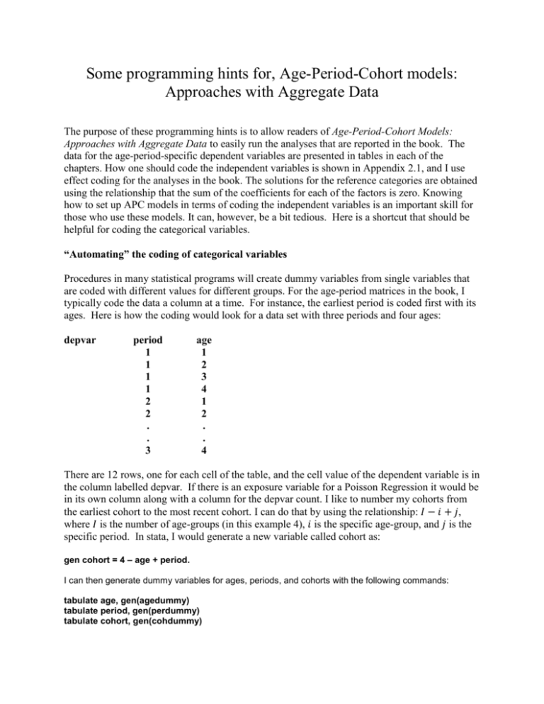
Some programming hints for, Age-Period-Cohort models:
Approaches with Aggregate Data
The purpose of these programming hints is to allow readers of Age-Period-Cohort Models:
Approaches with Aggregate Data to easily run the analyses that are reported in the book. The
data for the age-period-specific dependent variables are presented in tables in each of the
chapters. How one should code the independent variables is shown in Appendix 2.1, and I use
effect coding for the analyses in the book. The solutions for the reference categories are obtained
using the relationship that the sum of the coefficients for each of the factors is zero. Knowing
how to set up APC models in terms of coding the independent variables is an important skill for
those who use these models. It can, however, be a bit tedious. Here is a shortcut that should be
helpful for coding the categorical variables.
“Automating” the coding of categorical variables
Procedures in many statistical programs will create dummy variables from single variables that
are coded with different values for different groups. For the age-period matrices in the book, I
typically code the data a column at a time. For instance, the earliest period is coded first with its
ages. Here is how the coding would look for a data set with three periods and four ages:
depvar
period
1
1
1
1
2
2
.
.
3
age
1
2
3
4
1
2
.
.
4
There are 12 rows, one for each cell of the table, and the cell value of the dependent variable is in
the column labelled depvar. If there is an exposure variable for a Poisson Regression it would be
in its own column along with a column for the depvar count. I like to number my cohorts from
the earliest cohort to the most recent cohort. I can do that by using the relationship: 𝐼 − 𝑖 + 𝑗,
where 𝐼 is the number of age-groups (in this example 4), 𝑖 is the specific age-group, and 𝑗 is the
specific period. In stata, I would generate a new variable called cohort as:
gen cohort = 4 – age + period.
I can then generate dummy variables for ages, periods, and cohorts with the following commands:
tabulate age, gen(agedummy)
tabulate period, gen(perdummy)
tabulate cohort, gen(cohdummy)
2
In stata these commands provide us with the dummy variables for ages, periods, and cohorts. They are
stored in stata’s data editor and can be used as any other variables. If you want effect coding, you need
to change the reference groups scores to minus ones. In stata we can do this using the following recode
commands:
recode agedummy1 agedummy2 agedummy3 agedummy4 (0 1 = -1) if age==4
recode perdummy1 perdummy2 perdummy3 (0 1=-1) if period==3
recode cohdummy1 cohdummy2 cohdummy3 cohdummy4 cohdummy5 cohdummy6 (0 1=-1) if
cohort==6
That is, it changes the dummy codes for 0 and 1 to – 1 if the observation is in the reference category.
You may want to change the names of these effect coded variables, so you do not mistake them for
dummy coded variable or you may want to create these as new variables. Those options are available.
Chapter 1: Introduction to the Age, Period, and Cohort Mix
Figure 1.2
Produced using Excel from the data in Table 1.2.
Chapter 2: Multiple Classification Models and Constrained Regression
Table 2.4
The results in Table 2.4 were produced from the data in Table 2.3. The coding of the
independent variables follows the pattern shown in the appendix for effect coding and the
reference categories were age 75-79, period 1975-79, and cohort 1945. See the note on the first
page of these hints on how to “automate” this coding. Remember to calculate the person years of
exposure from Table 2.3 as noted in the first paragraph on page 34 when you are using Poisson
regression. When using OLS regression remember to take the natural logs of the rates; for
example, ln(0.44), ln(1.69), and so on.
Stata was used to produce all of the results. For example, I used the regular Poisson Regression
Program in Stata to produce the age1=age2, per2=per3 and coh6=coh7 results. The strategy I
used was to employ the generate command in stata to make these constraints; for example, gen
age1_2 = age1 + age2. Then I used stata’s Poisson command with age1_2 instead of age1 and
age2. The estimated coefficient for age1_2 is the constrained estimate for both age1 and age2.
The reference category coefficients are found easily since the sum of the coefficients for each
factor must equal zero if we use effect coding (I sum the coefficients for a factor such as age
from the output and the reference category must be minus this sum). Here is the Poisson
program for the age1=age2 constraint:
3
poisson brestcan age1_2 age3 age4 age5 age6 age7 age8 age9 age10 per1 per2 per3 per4
coh1 coh2 coh3 cob4 coh5 coh6 coh7 coh8 coh9 coh10 coh11 coh12 coh13 coh14,
exposure(exposurebc)
brestcan is the age-period-specific number of breast cancer deaths and exposurebc is the
computed number of person-years of exposure. Calculated from the data in Table 2.3.
As an important note; I am using age1 through age10 and per1 through per4 and coh1 through
coh14 generically. Your coding will differ if you use different names for your categorically
coded variables for ages, periods, and cohorts.
The intrinsic estimator’s coefficients are based on an online stata add-on program apc_ie. This
program can be accessed in stata by typing the command findit apc_ie and then the program and
help file can be downloaded.
The instructions for the use of this add-on are included in the help file. These should be read for
help in the coding of age, period, and cohort which are straight forward. The code we used to
generate the Poisson results in Table 2.4 for the intrinsic estimator is:
apc_ie brestcan, age(age) period(period) cohort(cohort) family(poisson) link(log)
exposure(exposurebc)
Table 2.5
We used the procedures employed in Table 2.4 to set the constraints. We used the log of the
rates from Table 2.3 for the dependent variable and used the regular regression procedure in stata
for the age, period, and cohort constrained solutions. For example, to set the age1 coefficient
equal to the age 2 coefficient, I used the generate command: gen age1_2 = age1 + age2. Then I
produced the age1=age2 results with the following regression analysis in stata:
regress lnratebc age1_2 age3 age4 age5 age6 age7 age8 age9 age10 per1 per2 per3 per4
coh1 coh2 coh3 cob4 coh5 coh6 coh7 coh8 coh9 coh10 coh11 coh12 coh13 coh14
For the intrinsic estimator we used the following code
apc_ie lnratebc, age(age) period(period) cohort(cohort)
Table 2.6
The procedures are the same as for table 2.4, except that this is run using dummy variable coding
for the independent variables. At least this is the case for the age1=age2, per2=per3, and
coh6=coh7 constraints. The intrinsic estimator is a bit more complicated. For the intrinsic
estimator, we obtain the result in Table 2.4 and then transform them according to the instructions
using the last paragraph on page 38 that continues on to page 41.
4
Table 2.7
The procedures are the same as for table 2.5, except that this run uses dummy variable coding for
the independent variables. At least this is the case for the age1=age2, per2=per3, and coh6=coh7
constraints. The intrinsic estimator is a bit more complicated. For the intrinsic estimator, we
obtain the result in Table 2.5 and then transform them according to the instructions using the last
paragraph on page 38 that continues on to page 41.
Figure 2.1 is made using Excel and the results from Table 2.5.
Table 2.8
The age-period model is just a regular regression with only the age and period effects (effect
coded). The dependent variable is the log of the breast cancer rate. The stata program is:
regress lnratebc age1 age2 age3 age4 age5 age6 age7 age8 age9 age10 per1 per2 per3 per4
I added zeros for the cohort effects, since they are assumed to be zero by being left out of the
model.
The zero linear constraint for cohorts is a bit trickier. In stata the constraint can be written as:
constraint 1 14*coh1 + 13*coh2 + 12*coh3 + 11*coh4 + 10*coh5 + 9*coh6 + 8*coh7 +
7*coh8 + 6*coh9 + 5*coh10 + 4*coh11 + 3*coh12 + 2*coh13 + 1*coh14 = 0
The constraint makes it so the resulting cohort coefficients do not trend over time. We then can
run a constrained regression in stata with this constraint:
cnsreg lnratebc age1 age2 age3 age4 age5 age6 age7 age8 age9 age10 per1 per2 per3 per4
coh1 coh2 coh3 coh4 coh5 coh6 coh7 coh8 coh9 coh10 coh11 coh12 coh13 coh14, c(1)
Table 2.9
The procedures used are described in the text, and the programming for the per2=per3 and
coh6=coh7 models has been described for Table 2.5.
Figure 2.3 (a, b, and c)
Programing for the constrained regression procedure has been described in the section for Table
2.8. The zero linear trend for periods has the following constraint for the data in Table 2.10:
Constraint 1 7*per1960 +6*per1965 + 5*per1970 + 4*per1975 + 3*per1980 + 2*per1985 +
1*per1990 = 0
Then one uses this constraint in a constrained regression for the logged age-period-specific
homicide rates to obtain the results graphed in Figures 2.3 (a,b, and c). The data for the
5
dependent variable are the logged age-period-specific rates in the body of Table 2.10; for
example, ln(8.98), ln(14.00), and so on. The independent variables are effect coded.
Chapter 3: Geometry of Age-Period-Cohort (APC) Models and Constrained
Estimation
All of the matrix results in Chapter 3 were calculated using Excel. This is a highly visual way
for students and researchers to picture what is going on in matrix algebra.
Table 3.3:
There is one table of results that used constrained regression: Table 3.3. From the examples in
Chapter 2 (see especially the discussion for Table 2.4 and Table 2.5), it should be clear how to
compute the constrained regressions for age1=age2, coh1=coh3, the intrinsic estimator, and the
zero linear trend for periods solutions. The data are from Table 3.2 and these age-periodspecific rates are logged; for example, ln(475), ln(366), and so on. The independent variables
are effect coded.
Chapter 4: Estimable Functions Approach
Table 4.3
Table 4.3 is based on the data in Table 4.2. The dependent variable is the logged value of the
age-period-specific differences in rates in Table 4.2. The independent variables are effect coded
and the analysis uses ordinary least squares regression. Again, to obtain the constrained
solutions for age1=age2 and coh1=coh2, we generate two new variable: gen age1_2 = age1 +
age2 and gen coh1_2 = coh1 + coh2. To compute the constrained solutions for cohort
coh1=coh2, for example, we regressed the log of the differences in rates on the age categorical
variables and the period categorical variables and all of the cohort categorical variables except
coh1 and coh2, which were replaced by coh1_2. Of course, these categorical variables do not
include the reference categories in our case age 80-84, period 2003, and cohort 1948-52. The
coefficient for coh1_2 is 1.485, and it is the coefficient for cohorts 1863-67 and 1868-72 in
Table 4.3.
To find the intrinsic estimator, we use the program apc_ie, described earlier in the programming
hints for Chapter 2. We use the version for OLS regression:
apc_ie depvar, age(age) period(period) cohort(cohort)
The values in the parentheses refer to the names you give to the variable that codes for ages, for
periods, and for cohorts and depvar is the name of the dependent variable (logged difference for
the lung cancer mortality rates in Table 4.2). The downloaded version of apc_ie is obtained by
6
typing findit apc_ie in the stata command line. Importantly, the help file associated with this
program will give instructions for coding of age, period, and cohort and for using the program.
To obtain the zero linear trend in periods estimates, we again use constrained regression in stata.
The constraint is:
constraint 1 11*per1 + 10*per2 + 9*per3 + 8*per4 + 7*per5 + 6*per6 + 5*per7 + 4per8 +
3*per9 + 2*per10 + 1*per11
I use per1 to per11 generically, you may designate your categorical cohort variables by different
names. As typical, these are effect coded.
To find the deviations from linearity in Table 4.3 for age, periods and cohorts I used the
following procedure (I outline the process for the age deviations from linearity). Find the linear
trend for the age coefficients by regressing the seven age coefficients (ordered from youngest to
oldest) on time (the numbers 1, 2, . . . , 7). We use these seven numbers because there are seven
age coefficients. The deviations from linearity are the residuals of these ages from their
predicted value given the slope. In stata we use these seven coefficients and these time trend
numbers as a data set. I used the regress command and regress these age coefficients on time.
After this regression run, I typed predict varname, residual in command line (varname is what
you want to name these deviations) to obtain the residuals (deviations from linearity). You can
follow the same procedure to find the trends and deviations from linearity for the period and for
the cohort coefficients. The trends differ from one constrained solution to another, but the
deviations from linearity remain the same.
Figure 4.1
This is an Excel produced graph based on the column of deviations from linearity in Table 4.3.
Chapter 5: Partitioning the Variance in Age-Period-Cohort (APC) Models
Table 5.1
We use the data from Chapter 2 (Table 2.3) for age-period-specific breast cancer mortality in
Japan. For the OLS analyses, we use the logged rates of breast cancer mortality (the table
includes non-logged rates). The analyses are described in the text. For the OLS results for
cohort, we use a single constraint that just identifies the model. For cohorts we exclude cohort 1.
The result is one of the infinite best fitting solutions. We compare this with the two-factor model
that contains all of the age and period coefficients, but none of the cohort coefficients. The
2
𝑅𝑖𝑛𝑐𝑟𝑒𝑚𝑒𝑛𝑡
is based on the difference between the 𝑅 2 for the two models. We obtained the F-test
for the increments by using stata’s test command. For cohorts, the stata code for the full APC
model is:
7
regress lnratebc a1 a2 a3 a4 a5 a6 a7 a8 a9 a10 p1 p2 p3 p4 c2 c3 c4 c5 c6 c7 c8 c9 c10 c11
c12 c13 c14
followed by the post estimation command test:
test c2 c3 c4 c5 c6 c7 c8 c9 c10 c11 c12 c13 c14
To find the 𝑅 2 for the two-factor (AP) model, I used the following stata command
regress lnratebc a1 a2 a3 a4 a5 a6 a7 a8 a9 a10 p1 p2 p3 p4
The analogous procedure was used for finding the unique effects of periods and ages.
To find the unique effects for the Poisson Regression for counts, we used a similar procedure.
Remember that the counts are derived from the data in Table 2.3 as described in the first full
paragraph on page 34 of the book. Here is an example stata coding for the effects of cohorts:
poisson brestcan a1 a2 a3 a4 a5 a6 a7 a8 a9 a10 p1 p2 p3 p4 c2 c3 c4 c5 c6 c7 c8 c9 c10 c11
c12 c13 c14, exposure(exposurebc)
followed by postestimation test command
test c2 c3 c4 c5 c6 c7 c8 c9 c10 c11 c12 c13 c14
The test command provides the Chi-square statistic and the associated probability. Using the
same general procedure, we estimate the unique effects for periods and ages.
Table 5.2
I am a bit embarrassed for there is a mistake in this table and in Figure 5.1 a. I will explicate
these below. Again I used stata to estimate these mixed effect models. To find the random
effects for cohorts, we use the age and period categorically coded variables as fixed level one
effects (excluding the reference variable categories) and cohort as the random effect. Cohort is
coded 1, 2, . . . , 15 from the earliest cohort to the most recent cohort. Of course, different cohorts
have different numbers of observations. The stata code is:
xtmixed lnratebc a1 a2 a3 a4 a5 a6 a7 a8 a9 a10 p1 p2 p3 p4 || cohort:,
covariance(independent) variance
To access the estimated random effect for each cohort, we use the post-estimation command
predict (where cohrandom is a variable name that I chose arbitrarily):
predict cohrandom, reffects
The random effects are used later for graphs
The fixed effects are part of the standard output for xtmixed as is the random variance associated
with the random factor.
8
For the Poisson mixed models, we use the command xtmepoisson. The example below involves
using periods as the random effect.
xtmepoisson brestcan a1 a2 a3 a4 a5 a6 a7 a8 a9 a10 c1 c2 c3 c4 c5 c6 c7 c8 c9 c10 c11 c12
c13 c14, exposure(exposurebc) || period:, covariance(independent) variance
Note that period is a variable that codes the five different periods as 1, 2, 3, 4, 5; the first to the
most recent period. To estimate the random effect for the individual periods, we again use the
postestimation command predict:
predict perrandom, reffects These are used later for graphs.
My error for the Poisson mixed models is that I did not use the option variance (I do so in the
example above). In Table 5.1 for the Poisson random variances, I reported random standard
deviations. The results using the variance should be
Random Variances
Cohorts
Periods
Cohorts
0.0069
0.0011
0.3354
Figures 5.1 (a,b,c)
These figures are based on the random effects that were generated by the post-estimation
command for the mixed models and the deviations of the coefficients for each factor from the
linear trend of each factor (based on OLS regression). See the last paragraph in the programming
hints for Table 4.3, for a description of how to calculate the deviations from linearity.
My error occurs in Figure 5.1a for the cohorts. I have the values reversed. The values for 1875
should be for 1945, the values for 1880 should be for 1940, and so on. The values for the linear
random effects are plotted correctly in Figure 5.3 a.
Figure 5.2 (a, b, and c)
These figures plot the fixed effects from the linear mixed model and for the corresponding two
factor models estimated using OLS. For example, the xtmixed model fixed effects for age and
period fixed effects (with cohorts as the random effect) and the OLS effects for an age-period
model where the cohort categorical variables are excluded are plotted in Figure 5.2a.
9
Figure 5.3 (a, b, and c)
These figures plot the random effects from the linear mixed model and from the Poisson mixed
model. These random effects for cohorts, periods, and ages were accessed using the postestimation command predict as described above (for Table 5.2).
Table 5.4
We move to an empirical example using homicide arrest data. Table 5.3 contains both the ageperiod-specific homicide arrest rates per 100,000 residents as well as the age-period-specific
number of arrests (in parentheses). The final sentence of the first full paragraph on page 136
explains how to compute the number of homicide arrests from the rate per 100,000 and the
number of homicide arrests. This is needed to conduct Poisson analyses for this data.
To test for the unique effects of age for the OLS results in stata use the following commands:
regress lnhom1564 age2 age3 age4 age5 age6 age7 age8 age9 period65 period70 period75
period80 period85 period90 period95 period00 period05 c1 c2 c3 c4 c5 c6 c7 c8 c9 c10 c11
c12 c13 c14 c15 c16 c17 c18
. test age2 age3 age4 age5 age6 age7 age8 age9
To find the increment in 𝑅 2 subtract the 𝑅 2 from a model with only the period and cohort
categorical variables from the 𝑅 2 for the full model (for example) the model with just one age1
excluded.
The same procedure provides the OLS Regression estimates of the unique effects for the other
factors in Table 5.4.
We use similar procedures for obtaining the estimates for the Poisson Regression of counts:
poisson homnumber age2 age3 age4 age5 age6 age7 age8 age9 period65 period70 period75
period80 period90 period85 period95 period00 period05 c1 c2 c3 c4 c5 c6 c7 c8 c9 c10 c11
c12 c13 c14 c15 c16 c17 c18, exposure(homexpsure)
To find Chibar2 and the probability value, we use the test post-estimation command
test age2 age3 age4 age5 age6 age7 age8 age9
Figures 5.4 (a, b, c, and d)
The observed rates by ages for each of these periods are in the data. The rates estimated using
age, period, and cohort can be produced from any of the analyses that contain the age, period,
and cohort categorically coded variables with a single just identifying constraint. They all fit the
data equally well and produce the same predicted values. After running such an analysis using
10
the regress command, one can retrieve the predicted values using the predict command. For
example,
predict estimates
where estimates is an arbitrary name I used for the predicted values.
To obtain the predicted values without cohorts, I ran an age-period regression without the cohort
categorically coded variables, and then found the predicted values for this model.
The plots were then constructed using excel.
Table 5.5
For these linear mixed models and Poisson mixed models, I used the same programing as
outlined for Table 5.2 using xtmixed and xtmepoisson.
For example, for the Poisson mixed model with cohorts as the random effect I used:
xtmepoisson homnumber age1 age2 age3 age4 age5 age6 age7 age8 age9 period65 period70
period75 period80 period85 period90 period95 period00 period05, exposure(homexposure)
|| cohornum:, covariance(independent) variance
predict cohortreffects,reffects
Figure 5.5 (a, b, and c)
I used the random effects obtained from the post-estimation commands to make the Excel
graphs.
Some calculations
I introduced the cohort characteristic approach early; it is covered in detail in the next chapter.
To run the mixed model with the cohort characteristics and cohorts as the random effect, the
cohort characteristics are simply added as fixed effects at level 1. This is how I obtained the
estimate for the cohort random variance in a model with cohort characteristics mentioned on
page 146 in the last full paragraph. The cohort characteristics appear in Table 7.1, a later
chapter. Not surprisingly they go with the cohort shown in the table. So there are two extra
columns in the data, one for each cohort characteristics. Each entry in the columns corresponds
to each observation and what is entered depends on the cohort for that observation.
Below is the code for the xtmepoisson procedure that includes the cohort characteristics:
lnillegit and lnrcs1564. We find the variance when cohort characteristics are included in the
model and the variance from a run when they are not included in the model:
11
xtmepoisson homnumber age1 age2 age3 age4 age5 age6 age7 age8 age9 period65 period70
period75 period80 period85 period90 period95 period00 period05 lnillegit lnrcs1564,
exposure(homexpsure) || cohornum:, covariance(independent) variance
Chapter 6: Factor-Characteristic Approach
For the empirical example in this chapter, I use the suicide data included in Tables 6.2 and 6.3.
Table 6.2 contains age-period-specific suicide rates per 100,000 and the two characteristics for
the cohorts. Table 6.3 contains the age-period-specific populations for use with Poisson
regression analyses. You simply enter the data you have into a data file: one observation for
1930, two for 1935, and so on. If you are using effect coding the final age category 70-74 is
coded with a -1, the period 2010 is coded with a -1 and the final cohort is coded with a -1. As
always the tables and analyses in the book use effect coding.
Table 6.4
For the OLS results, I simply regress the logged age-period-specific rates on ages and period and
then on ages, periods and cohorts. We use the following two stata commands:
regress lntotsui age1 age2 age3 age4 age5 age6 age7 age8 age9 age10 age11 age12 per1 per2
per3 per4 per5 per6 per7 per8 per9 per10 per11 per12 per13 per14 per15 per16
and for the cohort characteristic model
regress lntotsui age1 age2 age3 age4 age5 age6 age7 age8 age9 age10 age11 age12 per1 per2
per3 per4 per5 per6 per7 per8 per9 per10 per11 per12 per13 per14 per15 per16 lnnmbtot
lnrcstot
Note that we take the logged values of the cohort characteristics.
For the Poisson regressions, I use the same procedure except I employ Poisson Regression
poisson numsuitot age1 age2 age3 age4 age5 age6 age7 age8 age9 age10 age11 age12 per1
per2 per3 per4 per5 per6 per7 per8 per9 per10 per11 per12 per13 per14 per15 per16,
exposure(population)
and
poisson numsuitot age1 age2 age3 age4 age5 age6 age7 age8 age9 age10 age11 age12 per1
per2 per3 per4 per5 per6 per7 per8 per9 per10 per11 per12 per13 per14 per15 per16
lnnmbtot lnrcstot, exposure(population)
12
Table 6.5
For the age-cohort and the age-cohort period-characteristic analyses in Table 6.5 the procedure
follows those in for Table 6.4. We use the categorical measures for ages and cohorts and use the
unemployment data for periods in Table 6.2 and the Vietnam Era dummy variable with the
periods 1965, 1970, and 1975 coded as one and the other periods coded as zero.
Table 6.6
For this model I use the age categorical variables and the cohort and period characteristics. I
show the coding for the results for the Poisson regression models for age alone and for the age
period-characteristic cohort-characteristic model.
poisson numsuitot age1 age2 age3 age4 age5 age6 age7 age8 age9 age10 age11 age12,
exposure(population)
poisson numsuitot age1 age2 age3 age4 age5 age6 age7 age8 age9 age10 age11 age12
lnnmbtot lnrcstot lnunemptot vietnam, exposure(population)
Chapter 7: Conclusions: An Empirical Example
I use the data in Table 7.1 throughout this chapter. Remember that all analyses are conducted
with the data for the first three cohorts considered to be missing. That is, we treat the entry for
those 60-64 in 1965 as missing, and the two for those 55-59 in 1965 and 60-64 in a1970 as
missing, and he three observations in for those 50-54 in 1965 and 55-59 in 1970 and 60-64 in
1975 as missing.
Table 7.2
There are alternative ways to make sure that the results exclude the observations from the first
three cohorts. This involves more than simply not including these three cohorts in the analysis,
since if you do so their observations will still be used in the calculation of age and period effects.
One way is to code these observations as missing. Another is to not code these observations at
all (this is what I suggested for the suicide data used in Chapter 6. For this data I coded all of the
data and then eliminated the first three cohorts data by using an if statement that says that says
only observations should be used if NMB is not coded as missing (!= is not equal in stata). The
code for this run follows shortly.
I ran a regular regression analysis with all of the period and age categorical variables and left out
cohorts 1 through 4. If we leave out only cohorts 1 through 3 the model is not identified. Then
13
to estimate whether the increment to R-square moving from the AP model to the APC model is
statistically significant we use stata’s test command as in the following coding:
regress lnhom1564 age1 age2 age3 age4 age5 age6 age7 age8 age9 period65 period70 period75
period80 period85 period90 period95 period00 period05 c5 c6 c7 c8 c9 c10 c11 c12 c13 c14 c15
c16 c17 c18 if lnillegit != .
(The period is the missing value in stata; this is why we write !=. in the regression statement above).
Note that c1, c2 and c3 are not in the analysis since the data associated with these variables
are missing. We exclude c4 to identify the model.
test c5 c6 c7 c8 c9 c10 c11 c12 c13 c14 c15 c16 c17 c18
We use a parallel process to generate the periods and ages unique effects in Table 7.2. For
example for the period results in Table 7.2
regress lnhom1564 age1 age2 age3 age4 age5 age6 age7 age8 age9 period70 period75 period80
period85 period90 period95 period00 period05 c4 c5 c6 c7 c8 c9 c10 c11 c12 c13 c14 c15 c16 c17
c18 if lnillegit != .
test period70 period75 period80 period85 period90 period95 period00 period05
Figure 7.1 (a, b, and c)
The procedure to calculate these deviations from the linear trends in the age coefficients, period
coefficients, and cohort coefficients is to first run a regression analysis with the age, period, and
cohort categorical variables with one constraint (for example excluding one of these categorical
variables from the regression run. Then to find the age deviations from the linear trend, regress
the age coefficients on the numbers 1 to 𝐼 where 𝐼 is the number of age categories. Then make
these your data for a stata run and regress the age coefficients on the numbers 1 to 𝐼. The easiest
way to get the deviations is to request the residuals using the predict command: predict
deviations, residuals. Do the same for the period coefficients and the cohort coefficients. The
results are the same no matter which constraint you use – these deviations are estimable
functions. I plotted the deviations using Excel.
Table 7.3
I ran a constrained regression with the age, period, and cohort categorical variables with the
constraint that age1=age2. I put the results in a column in Excel. I put the null vector for these
data in another column of Excel. Now I simply choose different values of 𝑠 to multiply the null
vector and add those results to the corresponding elements to the age1=age2 constrained
solution. Someone with a moderate grasp of Excel can make this process streamlined. You can
set up formulas to produce a new solution vector that lies on the line of solution when you
change 𝑠. I did this and changed 𝑠 until I found a solution (labelled age4=age5) in Table 7.3,
where there is a just barely a monotonic drop in the age effect from its peak and for ages 30-34 to
14
35-39 and older (age4 is almost equal to age 5, but slightly higher). I then manipulated 𝑠 until
age1 was equal to age 3. I wanted for one boundary condition to have those aged 15-19 to have
a rate no higher than that for those 25-29. The best substantive solution was set based on what I
thought to be a reasonable age curve (my best guess as a criminologist). It is not the most
important of these age curve – the most important are the boundary age-curves.
Figure 7.2 (a, b, and c).
Figure 7.2a is the plot of the age curve based on these age boundaries and the “best substantive
estimate.”
Figure 7.2b is the plot of the period curve based on these age boundaries and the “best
substantive estimate.”
Figure 7.2c is the plot of the cohort curve based on these age boundaries and the “best
substantive estimate.”
Table 7.4
The first column of results is based on a simple regression analysis of the logged age-periodspecific homicide rates on the age and period effect coded categorical variables. The second
column of results is based on the regression of the logged age-period-specific homicide rates on
the age and period effect coded variables and the two cohort characteristics. The code for the run
for this second column is:
regress lnhomicidemissing age1 age2 age3 age4 age5 age6 age7 age8 age9 period65
period70 period75 period80 period85 period90 period95 period00 period05 lnrcs1564
lnillegit
Figure 7.3 (a, b, and c)
In Figures 7.3a and b we have plotted the results from the two models in Table 7.4 first for ages
(7.3a) for ages and then for periods (7.3b). The text (footnote on page 194) describes how we
calculated the cohort effects in Figure 7.3c.
Figures 7.4 (a,b, and c)
These figures are based on the results in Table 7.3 and the final column of results in Table 7.4.
Please feel free to comment on these notes. I would be happy to improve them. My e-mail
address i: bobrien@uoregon.edu.