F: Use the two-sample z procedures to give a confidence interval for the difference 𝑝
1
− 𝑝
2
between proportions in two populations.
G: Use a two-proportion z test to test the hypothesis 𝐻
0
two distinct populations are equal.
: 𝑝
1
= 𝑝
2
that proportions in
H: Check that you can safely use these z procedures in a particular setting.
Combined sample proportion
𝟏
𝟐
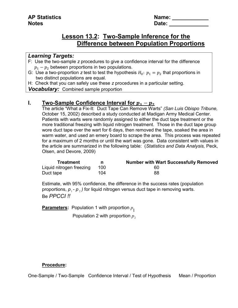
The article “What a Fix-It: Duct Tape Can Remove Warts” (San Luis Obispo Tribune,
October 15, 2002) described a study conducted at Madigan Army Medical Center.
Patients with warts were randomly assigned to either the duct tape treatment or the more traditional freezing with liquid nitrogen treatment. Those in the duct tape group wore duct tape over the wart for 6 days, then removed the tape, soaked the area in warm water, and used an emery board to scrape the area. This process was repeated for a maximum of 2 months or until the wart was gone. Data consistent with values in the article are summarized in the following table: ( Statistics and Data Analysis, Peck,
Olsen, and Devore, 2009)
Treatment n
Liquid nitrogen freezing 100
Number with Wart Successfully Removed
60
Duct tape 104 88
Estimate, with 95% confidence, the difference in the success rates (population proportions, p
1
- p
2
) for liquid nitrogen versus duct tape in removing warts.
Be
Parameters: Population 1 with proportion
Population 2 with proportion p
1 p
2
Procedure:
One-Sample / Two-Sample Confidence Interval / Test of Hypothesis Mean / Proportion

Samples: Choose a SRS separately from each population, or from each treatment group, if conducting a randomized comparative experiment.
Sample 1 has size
Sample 2 has size n
1
and sample proportion n
2
and sample proportion
ˆ
1
.
ˆ
2
.
Sampling Distribution of
ˆ
1
 p
2
: Mean:

ˆ
1
 ˆ p
2
=
 p
1
  p
2
= p
1
 p
2
Variance:
 2 p
1
 ˆ
2
=
 2 p
1
  2
2
= p
1
( 1
 n
1 p
1
)
 p
2
( 1
 p
2
) n
2
Standard Deviation:

ˆ
1
 ˆ p
2
= p
1
( 1
 p
1
)
 n
1 p
2
( 1
 p
2
) n
2
Conditions: S Two independent SRSs of sizes n and
1 n
2
drawn from two distinct
populations. Independent samples means one sample has no
influence on the other.
I Independent observations. Check if sampling without replacement.
Each population must be at least 10 times as large as its
corresponding sample

N
1

10 n
1
and N
2

10 n
2
.
N The sampling distribution of n
1
( 1 p
1
 ˆ
2
is approximately Normal if counts of “successes” and “failures” in both samples are at least 5  n
1 1

5 ,
 ˆ
1
)

5 , n
2 2

5 , and n
2
( 1
 ˆ
2
)

5 .
Calculations: Estimate the difference in the population proportions, p
1
- p
2 with 95% confidence.
Estimate

z

Standard Error of the Estimate
,
(
ˆ
1
 ˆ
2
)
 z
*
ˆ
1
( 1
 n
1
ˆ
1
)

ˆ
2
( 1
 n
2
ˆ
2
)
Interpretation: (Interpret results in context of problem.)

1
2
Do the data suggest that freezing is less successful than duct tape in removing warts?
Parameters: p
1
= p
2
=
Hypotheses:
H :
0
H : a
Procedure:
One-Sample / Two-Sample Confidence Interval / Test of Hypothesis Mean / Proportion
Samples: Sample 1 has size
Sample 2 has size n
1
and sample proportion n
2
and sample proportion
ˆ
1
.
ˆ
2
.
Note that in H
0 the claim is made that p
1
 p
2
, and thus the two population proportions equal some common population proportion, p c
. To estimate this common population proportion, we will use a combined sample proportion defined as follows: 𝑝 𝑐
= 𝑛
1 𝑝
1 2 𝑛
1
+ 𝑛
2
= 𝑡𝑜𝑡𝑎𝑙 𝑜𝑓 𝑠𝑎𝑚𝑝𝑙𝑒 𝑠𝑢𝑐𝑐𝑒𝑠𝑠𝑒𝑠 𝑡𝑜𝑡𝑎𝑙 𝑜𝑓 𝑠𝑎𝑚𝑝𝑙𝑒 𝑠𝑖𝑧𝑒𝑠
Use
ˆ c
in place of
ˆ
1
and
ˆ
2
in conditions and calculations of standard error.
Conditions: S Two independent SRSs of sizes n and
1 n
2
drawn from two distinct
populations.
I Independent observations. Check if sampling without replacement.
Each population must be at least 10 times as large as its
corresponding sample

N
1

10 n
1
and N
2

10 n
2
.
N The sampling distribution of p
1
 ˆ
2
is approximately Normal if counts of “successes” and “failures” in both samples are at least 5  n
1 c

5 , n
1
( 1
 c
)

5 , n
2 c

5 , and n
2
( 1
 c
)

5 .

Calculations:
Test Statistic: z

(
 ˆ
1 c
( 1
 n
1
2
) c
)


( p
1
 c
( 1 p
2
 n
2
) c
)
P-Value: P
Interpretation:
-value = P( z ) (Sketch required!!)
(Interpret results in the context of the problem.)