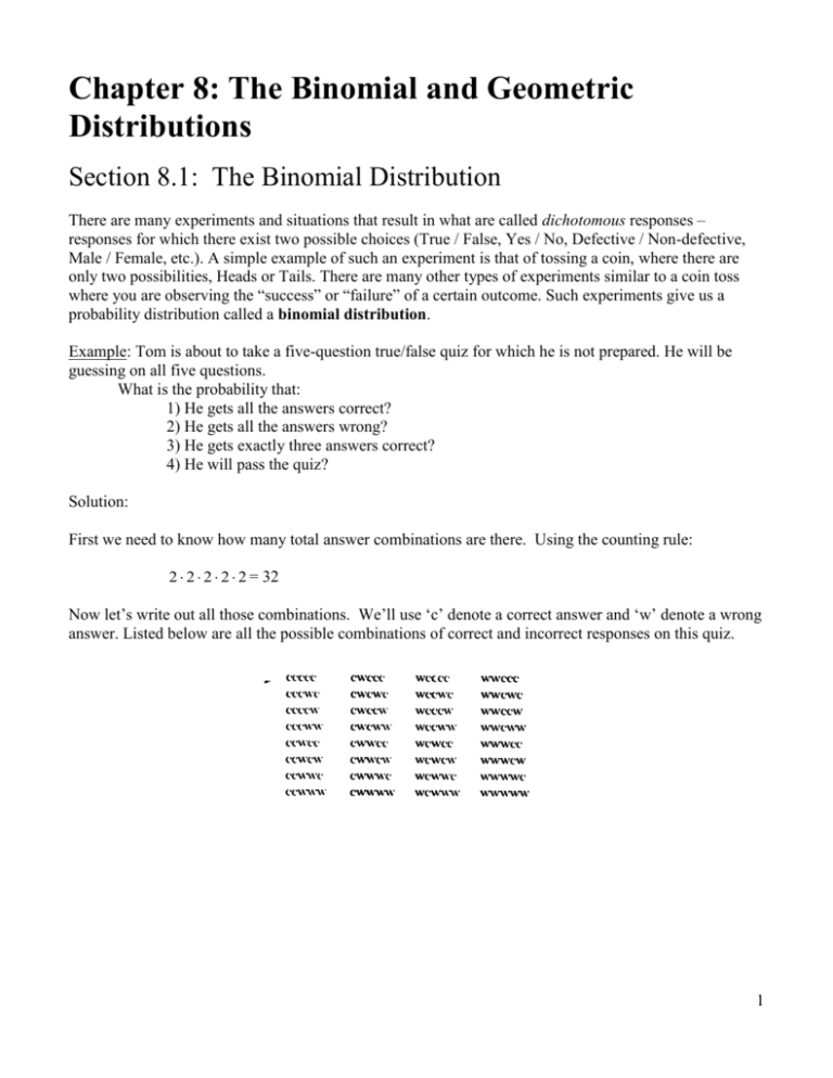
Chapter 8: The Binomial and Geometric
Distributions
Section 8.1: The Binomial Distribution
There are many experiments and situations that result in what are called dichotomous responses –
responses for which there exist two possible choices (True / False, Yes / No, Defective / Non-defective,
Male / Female, etc.). A simple example of such an experiment is that of tossing a coin, where there are
only two possibilities, Heads or Tails. There are many other types of experiments similar to a coin toss
where you are observing the “success” or “failure” of a certain outcome. Such experiments give us a
probability distribution called a binomial distribution.
Example: Tom is about to take a five-question true/false quiz for which he is not prepared. He will be
guessing on all five questions.
What is the probability that:
1) He gets all the answers correct?
2) He gets all the answers wrong?
3) He gets exactly three answers correct?
4) He will pass the quiz?
Solution:
First we need to know how many total answer combinations are there. Using the counting rule:
2  2  2  2  2 = 32
Now let’s write out all those combinations. We’ll use ‘c’ denote a correct answer and ‘w’ denote a wrong
answer. Listed below are all the possible combinations of correct and incorrect responses on this quiz.
1
If we wanted to make a probability distribution for this situation we would place the above outcomes into
a table like the one below, and then make a probability distribution table (X = number of correct
responses):
x
0
1
2
3
4
5
p(x)
1/32
5/32
10/32
10/32
5/32
1/32
Using the probability distribution, we can now answer the questions posed:
1) The probability that Tom gets all the answers right is 1/32
2) The probability that Tom gets all the answers wrong is 1/32
3) The probability that Tom gets exactly 3 problems right is 10/32
4) The probability that Tom passes the quiz is the probability that he gets a 60 or above which is
the probability that he gets at least 3 question correct which is 16/32
The first two questions we can answer using our old probability methods, but the third and fourth require
the more elaborate analysis.
This long process can be avoided by using the notion that this is a binomial probability distribution. There
is a formula we can use to find the probability of any value in a binomial distribution:
P( x) 
n!
 p x  q n x
(n  x)! x!
for x  0,1, 2, 3, ...., n
n = # of trials
x = # of successes among n trials
p = probability of success in any one trial
q = probability of failure in any one trial (q = 1 – p)
2
Let’s apply the binomial probability information to Tom’s true/false test, Question 3:
First we need to define “success” to mean getting a question correct, and “failure” as getting a question
incorrect.
Next we need to find the values for n, x, p, q, and P(x).
n = 5 (there are 5 questions on the test which Tom can answer correctly or incorrectly)
x = 3 (Out of the choices 0,1,2,3,4,5, we are looking for the one where x=3)
p = .5 (The probability of “success”, i.e that Tom will get a question correct, is .5)
q = .5 (the probability that Tom will not get a question correct is 1-.5 = .5)
P(x) = We specifically are looking for p(3), i.e the probability that Tom will have exactly 3 “successes”
Having all the given information, we can find:
P(3) 
5! .53.553  10  03125
.
(5  3)!3!
32
To answer question four we would need to use the above method to find P(3), P(4), and P(5) and add
them all up.
This process can become tedious, which is why our calculator has a binomial function built in to make
your life easier. The syntax is: Binompdf(n, p, X) or Binomcdf(n, p, X) The latter adds up the individual
probabilities from 0 to X to give you the probability of less than or equal to X. So for the last question
you would do 1 – binomcdf(5, .5, 2).
Like all probability distributions, the binomial distribution has a mean,  and a standard deviation . The
formulas for finding these values are quite simple:
  np
 2  np (1  p )
  np (1  p )
3
Example 1: Suppose Charlie manages to manipulate a coin in such a way that it lands on heads with a .7
probability and lands on tails with a .3 probability. Suppose John then flips the coin 20 times, what is the
probability that it will land on heads for exactly 13 of the twenty flips? On average, how many flips will
result in a heads? What is the standard deviation of this binomial distribution?
Example 2: Suppose that the probability that any random freshman girl will agree to go with Sam to the
senior prom is 0.1. Suppose Sam asks 20 random freshman girls to the prom, what is the probability that
exactly 1 will say “yes”? That at least 1 will say “yes”? On average, how many freshman girls will agree
to go with Sam to the prom? What is the standard deviation of this binomial distribution?
4
Section 8.2: The Geometric Distribution
Let’s start with a simulation: Roll a die until the number six appears and keep a record of how many
rolls it took before the six was obtained.
While in a binomial distribution the random variable was the number of successes in a fixed number of
trials, in a geometric distribution the random variable is the number of trials it takes to achieve a
success.
Examples:
1) flip a coin until you get heads
2) Roll a die until you get a 6
3) Throw darts at a dartboard until you hit the bull’s-eye
A geometric distribution must have the following properties:
1) Each trial in the experiment must have only two possible outcomes (success or failure)
2) The probability of success, p, doesn’t change from trial to trial
3) The trials in the experiment are independent
4) The variable of interest is the number of trials required to reach the first success.
Example: We will take our simulation example to analyze various aspects of the geometric distribution.
Lets first find the various probabilities associated with our dice simulation and come up with a probability
distribution:
a. The probability that a 6 will come up on the first roll is (1/6) so for X = 1, P(X) = 1/6
b. The probability that a 6 will come up on the second roll is the probability that it WON’T come
up on the first roll AND that it WILL come up on the second roll.
Let i = P(won’t come up on the first roll) = 5/6
Let ii = P(will come up on the second roll = 1/6
So since events i and ii are independent P(i AND ii) = P(i) X P(ii) = 5/6 X 1/6 = 5/36
c. The probability that a 6 will come up on the third roll is the probability that it WON’T come up
on the first roll AND that it WON’T come up on the second roll AND that it WILL come up on
the third roll.
Again, since all three events mentioned are independent, we can find the probability that the first
and second and third will occur to be (5/6) X (5/6) X (1/6) = 25/216
5
d. If we proceed in the manner above will come up with the following probability distribution:
X
P(X)
1
1/6
2
5/61/6
3
5/65/61/6
4
5/65/65/61/6
5
5/65/65/65/6
1/6
n
(5/6)n-1(1/6)
e. We can generalize from the table above that for any geometric distribution:
P(X = n) = (1-p)n-1p
where p = probability of success
f. The mean, , of a geometric distribution (the average number of times we can expect to repeat
the trials before a success occurs) is simply 1/p where p is the probability of success.
Therefore for our example  = 1/(1/6) = 6. So we can expect, on average to roll the die 6 times
before getting the number 6.
g. The probability that it takes more than n trials to see a success is:
P(X>n) = (1 –p)n
So in our example the probability that it would take more than 10 rolls for us to get the number 6
is (1- (1/6))10 = 0.1615
h. The variance of a geometric distribution var(X) = (1 - p) / p2
In our case the variance is Var(X) = (1-1/6)/(1/6)2 = 25
6