Provisional translation
ONE. GENERAL PROVISION
The purpose of this guideline is to give knowledge of general statistical and mathematical
modeling tools that are used to calculate operational risk to bank employees and supervisors.
TWO. RISK ESTIMATION PRINCIPLE
All models that included in this guideline are based on conditional (Bayesian) and
unconditional (Frequentist) probability theory and philosophy. When choosing the usage of
above principles, banks and financial institutions shall consider their operations’ uniqueness.
THREE UNCONDITIONAL PROBABILITY MODELS
3.1.Risk estimation principle
It is common to use random discrete variables in calculating operational risk. Thus it is
very important to pay attention to the frequency of the data and the expected loss when
calculating operational risk.
Primary principle of calculating operational risk using unconditional probability is to find
probability distribution of the random variable that is consistent with loss data. Commonly
applied probability distributions for risk estimations are included in the Annex 1 of this
guideline. Review of consistency of loss data with the probability distribution of random
variable is evaluated according to 3.2 of this guideline.
3.2. Choosing a probability distribution for the risk estimation
Following tests statistics show the degree of consistency of loss data with common
probability distributions:
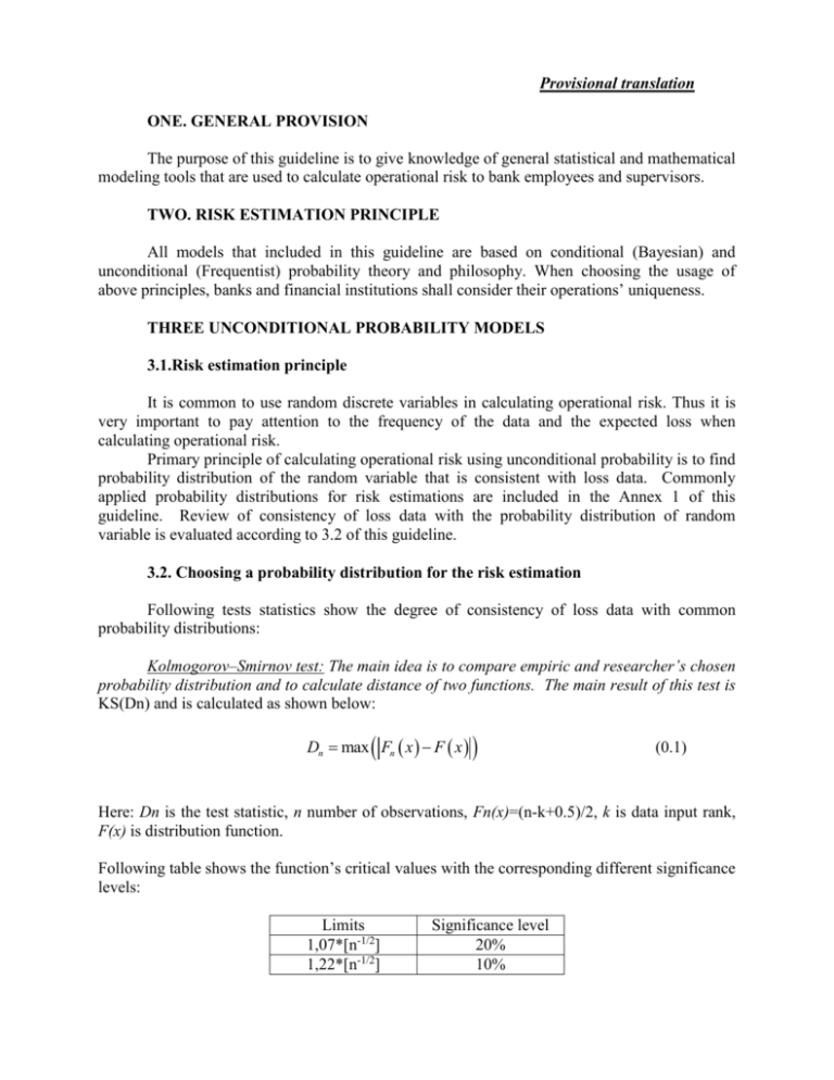
Kolmogorov–Smirnov test: The main idea is to compare empiric and researcher’s chosen
probability distribution and to calculate distance of two functions. The main result of this test is
KS(Dn) and is calculated as shown below:

Dn  max Fn  x   F  x 

(0.1)
Here: Dn is the test statistic, n number of observations, Fn(x)=(n-k+0.5)/2, k is data input rank,
F(x) is distribution function.
Following table shows the function’s critical values with the corresponding different significance
levels:
Limits
1,07*[n-1/2]
1,22*[n-1/2]
Significance level
20%
10%
1,36*[n-1/2]
1,63*[n-1/2]
5%
1%
Kolmogorov–Smirnov test is deemed statistically weak because it chooses the maximum value of
distance of associated functions. Disadvantages of Kolmogorov-Smirnov test is more noticeable
in samples with small number of observations.
Anderson-Darling test: This test is advanced version of the Kolmogorov-Smirnov test.
Following method is used to calculate the test statistics.
An2  


Fn  x   F  x    x  f  x  dx
2
(0.2)
Here:

n
F  x  1  F  x  
(0.3)
n- is the number of observations, F(x) is researcher’s chosen probability distribution function,
f(x) is probability distribution density function where Fn(x) =(n-k+0.5)/2. Following are critical
values of test statistics:
Size
1+0,2*[n-1/2]
1+0,3*[n-1/2]
At 5% significance level At 1% significance level
0.757
0.05
1.321
0.01
This test statistic is more robust than Kolmogorov-Smirnov test in that it considers all possible
distances calculated across vertical axis, with a help of  function distribution variance is
neutralized, also with a help of distribution density, the difference between the functions are
weighed with their corresponding probabilities.
Kramer Fon Mises test: It is a statistical test that calculates distance between the
functions, from which the square average is derived and compared. The indicator is calculated as
follows:
2
1
W 2    F  x   Fn  x   
(0.4)
12n
Kramer Fon Mizes test is unique in that the test is adjusted with its number of
observations. Following are critical values of test statistics:
Size
1+0,2*[n-1/2]
1+0,16*[n-1/2]
At 5% significance level At 1% significance level
0.124
0.174
0.222
0.338
3.3.Risk estimation using extreme value distribution
It is common knowledge that operational risk data is limited; also it is not effective to use
normal distribution and other similar distributions due to the fact that value of loss is very high if
loss event is occurred. Thus researchers, in that situation, prefer to use distribution of extreme
values rather than using whole distribution. “Frechet”, “Gumbel”, and “Weibull” distributions
are frontrunners of extreme value distribution.
Since extreme value distribution and its similar theories cover broad range of topics, it is
better to present the core ideas and summaries.
Theoretical part: For distribution function FR defined in interval (l, u), with random
values R1 , R2 Rn , the extreme values Zn is defined as follows:
Zn  Min  R1 , R2
Rn  эсвэл Zn  Max  R1 , R2
Rn 
(0.5)
If sample values in FR distribution are independent, distribution of random values Zn can be
shown as follows:
FZn ( z)  1  1  FR  z  
n
(0.6)
Due to the problems that occur by using formula (1.6) directly, the nomralization  Zn  n  n is
incorporated with parameters n indicating scope and n indicating location to the formula. The
formula after normalization is shown below:

FZ  z   1  exp  1   z 
1

(0.7)
where “ “ is called the index indicating the “tail” of the distribution. If (  >0), then (1.7) is of
“Weibull”, if ( =0) then (1.7) is of “Gumbel” and if ( <0) then (1.7) is of “Frechet” shape of
distribution.
VaR risk calculation: Building on the theoretical part of this guideline and extreme value
theory, the value at risk (VAR) concerning the operational risk of an institution at a certain
significance level can be assessed as:
p ext
1
 
 




VaR


asymp
n

 1  FZn  VaR   exp  1   
  
 

n

  

(0.8)
By manipulating (1.8), we can calculate the unexpected loss as follows:
VaR    n 
n 
ext  
1


ln(
p
) 


 
(0.9)
Parameter estimation: As there are many ways to calculate parameters of (1.9), let us
apply the moment method of (1, 2, 3 ….)th order. If we denote the moment of order “r” as “mr”,
for “n” number of observation and Xj random variable the moment is defined as follows:
mr 
1 n
X jU rj

n j 1
(0.10)
Where Uj is independent from F(Xi) distribution and is defined by formula pj=(n-j+0.5)/n.
According to Hoskings’ calculation (Hosking 1985), distribution moments can be represented
using associated parameters:
mr 

1 
 n  n
r 1 


  1    

1 
 
 1  r  
  1,  0
(0.11)
Iteration method is used for parameter estimation based on (1.11) which in turn brings numerous
problems. Thus in order to simplify the complexity, Hosking proposed the following formulas to
calculate parameters:
n 
 2m
2

 m1 
 1    1  2 
 n  m1 
n
1   1    

  7.859c  2.9554c 2
c
2m2  m1
3m3  m1

ln(2)
ln(3)
(0.12)
(0.13)
(0.14)
(0.15)
Example: The table below shows the amount of missing cash assets or the assets at the
branch of Bank A due to the illicit activities (fraud):
Year
1992
1993
1994
1995
1996
1997
1998
1999
2000
2001
2002
2003
Deficit
250,000.00
201,600.00
199,000.00
182,000.00
182,000.00
175,000.00
165,200.00
160,300.00
150,000.00
110,000.00
100,000.00
95,000.00
Based on the information above, the parameters of interests and the amount of
operational risk are:
c  0.0481732   0.3854517
 n  44, 698.36  n  111, 209.94
Based on value of parameters, the unexpected loss from the operational risk equals
VAR =204,161.91. We used pext=0.01 for the loss calculation.
3.4.Risk model, calculation validation
There are many methods to validate risk model used in risk estimation with actual
outcomes. Of these methods, the simplest and widely used one is calculating the share of
number of excess of actual loss over the projected loss. In other words, in actuality there are
instances where the actual loss is significantly higher than the projected loss using mathematical
and statistical tools raising the question to modify or change the existing model.
Besides simple ratios, there are many modern approaches that are based on statistical
theories. For the purpose of informing, Kupier test, included in Basel committee documents, is
introduced below.
As the test statistic states for “T” number of observations, “V” number of occurrences that
actual loss exceeded the projected loss, the associated probability equals (1  p)T V pV . If null
hypothesis is Ho: p=p* (here p* is significance level) test statistics is defined as below:
LRUC
 T T V  V V 
* T V
*V 

 2 ln 1  p 
p   2 ln 1     


 V   T  
(0.16)
Here LRUC has 2(1) distribution and if LRUC>3.84 hypothesis is cancelled. In other
words if LRUC<3.84, then the model has to be changed or modified.
FOUR. CONDITIONAL PROBABILTY MODELS
4.1.Background
It is common to have few or nonexistent quantitative data available for operational risk
estimation. In those cases it is only recommended to use simulation method to derive quantitative
data. Bayesian statistics calculation widely uses simulations based on conditional probability,
and this makes it very suitable for operational risk estimation.
One drawback to Bayesian statistics calculation is that it considers many subjective
factors, which makes it questionable for some researchers. Such disagreements usually caused
by different use of statistical terms, and goal of statistics is not clearly defined. For example,
many people argue on the term “parameter distribution” and “probability distribution.”
4.2.Theoretical part
Let’s suppose statistics model is aimed to define states of vector yt that consist of
random variables with p 1 dimension. Here the notation “t” depending on condition it can
define time, space, observation unit and etc. Let’s suppose Yt   ys s 1 shows the first t
t
observation of the sample. Also  is yt ’s sample set, where Yt’s sample set is  and
 0  0   . In this case “A” statistical model can represent a sequence of density functions
in following way:
p  yt Yt 1 ,  A , A 
(0.17)
Here A is k A 1 dimensional vector which contains unknown random variables where
 A   A  k has to be satisfied. The specification of A- depends on the choice of the model.
For example, for the most econometric models, A is unknown parameters or latent variable.
A
p( . ) is v( . ) dimensional density function. The dimension v( . ) determines whether the
random variable is discrete or continuous.
Using condition of the model “A” model and A unknown vector, we can define density of the
Yt:
T
p YT  A , A    p  yt Yt 1 ,  A , A 
(0.18)
t 1
If, for a given model, there is no relation between yt vectors, then;
p  yt Yt 1 ,  A , A   p  yt  A , A 
(0.19)
In this case it is:
T
p YT  A , A    p  yt  A , A 
(0.20)
t 1
As (1.18) and (1.20) only defines part of the model, we need to take into account the concept of
the prior density to get the general picture of the model. Prior density p(A|A) is the set of
quantifiable numbers that belongs to A vector consistent with the “A” model. In other words,
p(A|A) containes A ‘s information before the information “y” is revealed.
By combining prior density and (1.18) we can get “y” and A’s general density equation:
p  y,  A A   p  A A  p  y  A , A 
(0.21)
At the same time we can show general density in a following way
p  y,  A A   p  y A  p  A y, A 
(0.22)
Thus by combining (1.21) and (1.22) we get:
p  A y, A  
p  A A  p  y  A , A 
p  y A
(0.23)
In reality, most of the time it is difficult to estimate p(y|A) and if the general form of p(A|y,A)
can be derived it is only possible to make conclusion Thus it is recommended to use following
simplified formula:
p  A y, A   p  A A  p  y  A , A 
(0.24)
Here p(A |y,A)’s density is posterior density. In conclusion the purpose of calculating p(A
|y,A) is to reach the unambiguous conclusion on a given unknown variable by combining one’s
prior knowledge with the number of observation.
4.3.Using Bayesian theory for risk estimation
For the most risk modeling, mean and deviation are of importance for conducting
researches and analysis. However, in reality, due to various reasons it is difficult to estimate
these parameters thoroughly.
For example, when calculating foreign currency risk using VaR method, exchange rate
fluctuation (unknown parameter) should be calculated. However factors such as political
instability, economic cycles, exchange rate regime, balance of payments, foreign currency
reserve, the outcome and the expectation for the foreign currency volatility can differ. In other
words, the final amount of loss is dependent on the chosen value for the foreign exchange
volatility.
This uncertainty causes difficulties for bank and financial institution management to
make prudent decisions on risks. For example: If a bank is to place capital to absorb the loss
from operation risks, it is difficult for banks to precisely determine the amount of loss due to the
uncertainty of the parameters
These statistical methods that are based on Bayesian theory tackle those problems very
well. This can be seen from the following formula:
p  y, A   
A
p   A , y, A  p  A y, A  dv( A )
(0.25)
Here: from previous example,  is an expected loss from exchange rate fluctuations, A is
currency volatility.
4.4. Choosing prior density
In Bayesian methods, final outcome depends on prior distribution choice. Thus, let us
discuss more about prior density.
One of the most commonly used prior density is “elicited prior”. In most cases it relates
to the predictions of experienced experts in a chosen field.
To determine unknown parameter’s expected values, so-called “uninformed prior” is
important. An example of this is distribution of random values with the same probability in (0,1)
interval. As regards “Uninformed prior” we shall discuss about “Jeffreys prior”-, because
“Jeffreys prior” tends to maintain its inherent characteristics even after some changes were
made.
“Conjugate prior” is a prior density which has similar function shape with (1.18) and
(1.20).
A prior density with some missing feature is called “hyperprior”. “Hyperpriors” can be
used as a combination, however we shall note that this raises uncertainty.
4.5. Bayesian sample method and parameter estimation
With the recent advancements in technologies and information processing, it is made
possible to actually calculate many Bayesian-based different methods. For purpose of examples
Markov Chain Monte Carlo (MCMC) methods are used below.
Models that based on Bayesian theories try to evaluate following formula:
E  f  x   
 f  x    x  dx
   x  dx
(0.26)
Here (x) is posterior distribution. Monte Carlo method tries to calculate E[f(x)] by sampling
specified numbers for (x).
1 T
E  f  x     f ( X t )
n t 1
(0.27)
However, since in reality it is common for (x) to be of non-standard distribution form, f it is
limited to sample numbers. The most common way of overcoming this problem is to use
Markov Chain series.
Gibbs sampler: It divides A parameter into following subsets:
'
'
   (1)
,  (2)
,...,  (' B ) 
(0.28)
′
′
′
′
𝜃<(𝑏)
= (𝜃(1)
, … . , 𝜃(𝑏−1)
) 𝑎𝑛𝑑 𝜃<(1)
= {∅}
(0.29)
′
′
′
′
𝜃(𝑏)>
= (𝜃(𝑏+1)
, … . , 𝜃(𝐵)
) 𝑎𝑛𝑑 𝜃(𝐵)>
= {∅}
(0.30)
Where for any b vector:
Similar to this
Considering (1.29) and (1.30) let’s put following formula:
 ' (b )   ' (b ) , ('b )  
(0.31)
For Gibbs method it is crucial when choosing number of subsets in (1.28), it should be


possible to sample density function through the conditional probability formula - p (b )   (b ) , I .
When this criteria is met, the initial sample value (0) is chosen from distribution density p( | I)
in a following way:
(0)'
 (0)'   (1)
,..., ((0)'
B) 
(0.32)
Next step is

(1)
(0)
((1)
b )  p  ( b )  ( b ) ,  ( b )  , I

(b  1,..., B)
(0.33)
(1)'
,..., ((1)'
Here  (1)   (1)
B )  . Following this principle with m steps

((bm) )  p (b ) ((mb)) ,((bm)1) , I

(b  1,..., B)
m  1, 2,3...
(0.34)
These steps forms {(m)} Markov chain and migration probability is formularized as follows:


B

p  ( m )  ( m 1) , G   p  ((bm) )  ( (mb)) , ((bm) 1) , I
b 1

(0.35)
Metropolis-Hastings Algorithm To define model parameters with a help of this algorithm,
any migration probability density function q(* | , H), the argument * that is the value
indicating density, initial values  (0)   that needed to start the calculation must be given
beforehand. In each step of the algorithm, the test whether the sample value * from

q  *  ( m1) , H

is compatible to (m) should be performed. This can be determined with
following probability:

  
*
 m 1
 
 


 p  * I / q  *   m1 , H



, H  min 
,1
( m 1)
( m 1)
*
I /q 
 ,H 
 p 




(0.36)
If the sample value * is incompatible with (m, it is inferred as (m) = (m-1)
To further elaborate the algorithm, the kernel (any non-negative, proportional to the given
density value) of the “approved” sample values of distribution density are defined as follows:

 
 
u * , H  q * , H  * , H

(0.37)
Also, the probability to reject the sample values is calculated as:


r  H   1   u  *  , H dv  * 

(0.38)
In other words, for any given , (1.38) is able to shows the probability that * is rejected and the
probability can be determined before sampling the *.
Thus, Markov chain related to this algorithm is extracted from migration probabilities defined at
“v” dimensional sets - A   in a following way:


P  A  , H    u  *  , H dv  *   r  H  I A  
A
(0.39)
Therefore, to define migration density, Dirac delta function  ( *) is calculated in a following
way:
    f   dv    f   I  
*
*
*
A
A
(0.40)
Based on this, (m-1) indexed Markov chain is defined as follows:

 
 

p  ( m)  ( m1) , H  u  ( m)  ( m1) , H  r  ( m1) H  ( m1)  ( m) 
(0.41)
REFERENCE
Arnold Zellner “Bayesian Econometrics” Econometrica March 1985
Arnold Zellner “Some Aspects of the History of Bayesian Information Processing” Conference
Paper Washington D.C 2003
Basel Committee on Banking Supervision “Basel II: International Convergence of Capital
Measurement and Capital Standards” A Revised Framework - Comprehensive Version, June
2004
Basel Committee on Banking Supervision “Operational risk transfer across financial sectors”
Joint Forum Report, November 2001
Basel Committee on Banking Supervision “Regulatory Treatment of Operational Risk” Working
Paper, September 2001
Basel Committee on Banking Supervision “Sound Practices for the Management and
Supervision of Operational Risk” Consultative Document, February 2003
Edward I. Altman, Anthony Saunders “An Analysis and Critique of the BIS Proposal on Capital
Adequacy and Ratings” NYU Salomon Center’s Stern School of Business Forum, February 2000
Edward T.Jaynes “Bayesian Methods, General Background” Fourth Annual Workshop on
Bayesian/Maximum Entropy Methods August 1984
Francois M.Longin “From value-at-risk to stress testing: The extreme value approach” Journal
of Banking and Finance 24 (2000) 1097-1130
Hennie Van Greuning, Sonja Brajovic Bratanovic “Analyzing and Managing Banking Risk:
Framework for Assessing Corporate Governance and Financial Risk” World Bank Publications;
2nd edition, May 2003
John Geweke “Contemporary Bayesian Econometrics and Statistics” Wiley Series in Probability
and Statistics 2005
Kai Li, David Weinbaum “The Empirical Performance of Alternative Extreme Value Volatility
Estimators” December 20, 2000
Karsten T.Hansen “Introduction to Bayesian Econometrics and Decision” January 2002
Marcelo G. Cruz “Modelling, measuring and hedging operational risk” Wiley Finance Series
2002
Paul Embrechts “Extreme Value Theory as a Risk Management Tool” April 1999
Paul Embrechts “Extreme Value Theory: Potential and Limitations as an Integrated Risk
Management Tool” January 2000
Sune Karlsson “Bayesian Methods in Econometrics: Numerical Methods” November 2004
Siddhartha Chib "Markov Chain Monte Carlo Methods: Computation and Inference" Handbook
of Econometrics: volume 5 (eds J.J. Heckman and E. Leamer)
North Holland, Amsterdam, (2001), 3569-3649.