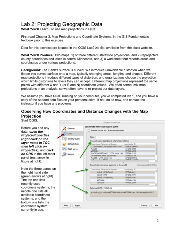
Lab 2: Projecting Geographic Data
What You’ll Learn: To use map projections in QGIS.
First read Chapter 3, Map Projections and Coordinate Systems, in the GIS Fundamentals
textbook prior to this exercise.
Data for this exercise are located in the QGIS Lab2 zip file, available from the class website.
What You’ll Produce: Two maps, 1) of three different statewide projections, and 2) reprojected
county boundaries and lakes in central Minnesota, and 3) a worksheet that records areas and
coordinates under various projections.
Background: The Earth's surface is curved. We introduce unavoidable distortion when we
flatten this curved surface onto a map, typically changing areas, lengths, and shapes. Different
map projections introduce different types of distortion, and organizations choose the projection
which limits distortions to levels they can accept. Different map projections represent the same
points with different X and Y (or E and N) coordinate values. We often cannot mix map
projections in an analysis, so we often have to re-project our data layers.
We assume you have QGIS running on your computer, you’ve completed lab 1, and you have a
copy of the needed data files on your personal drive. If not, do so now, and contact the
instructor if you have any problems.
Observing How Coordinates and Distance Changes with the Map
Projection
Start QGIS.
Before you add any
data, open the
Project-Properties
(right click on the
layer name in TOC,
then left click on
Properties), and click
on CRS in the left-most
panel (rust arrow in
figure at right).
Note the three panes on
the right hand side
(green arrows at right).
The top one lists
recently used
coordinate systems, the
middle one lists all
available coordinate
systems, and the
bottom one lists the
coordinate system
currently in use.
1
Although it depends on your settings, a new project will often default to the WGS84 coordinate
system before you’ve added any data.
Note the filter option near the top. This filters the available coordinate systems by a phrase, e.g.,
entering “UTM” there would only list coordinate systems with UTM in their name.
Also note the “Hide deprecated CRSs” check box near the middle-right. This should usually be
checked when you are selecting new coordinate systems, to not list “obsolete” coordinate
system versions.
Finally notice that each listed coordinate system has an “Authority ID”, typically a 4- or 5-digit
number. You can use these numbers as shortcuts when filtering or specifying coordinate
systems.
-Close the Properties panel and inspect the lower righthand corner of the main QGIS window. Notice the
EPSG:4326 in the lower right? Your number might be
different, depending on the default or selected coordinate
system. This is the current coordinate system, denoted
by its Authority ID. Also note the circle with a pattern
inside just to the right of the EPSG number. This is a
shortcut button to the CRS menu you just displayed through Project-Properties.
Any data that is suitably documented and is added to a project window is usually converted to
that window’s coordinate system “on the fly”. This means the coordinate projection is applied to
the data read from the disk, but before it is displayed. This projection is “temporary” in that it
doesn’t affect the data stored on the disk – it only reprojects the data temporarily, for display.
This allows us to display many data sets even if the data sets are stored in different map
projections, without having to go to the trouble of manually reprojecting each data set and
saving a new version of the data set. We can mix data stored in different coordinate systems,
e.g., a state plane system and a UTM system, without the data misaligned.
This automatic “on the fly” reprojection can be dangerous, though, because many spatial
operations will be in error when applied to data in different coordinate systems. Some
operations automatically reproject the data into the same coordinate system before applying the
operation, some don’t. You may get the impression the data are in the same coordinate system
when you display them together because you have “on the fly” reprojection set. However, they
may not be, and your spatial operation won’t work, and you’ll wonder why.
When you first create a project window, the coordinate system may be set to a default you may
not want, or it may be undefined. All subsequent data are then displayed in this “first” coordinate
system, unless you explicitly set this data frame coordinate system.
-Select Project-Properties from the main menu/dropdown menu, and click on CRS to open
the projection window again.
2
Note the check box
along the top edge
labeled “Enable ‘on
the fly’ CRS
transformation.”
We will use this in the
next few steps to
change the CRSs for
the display, and view
how they affect the
displayed shape of our
data.
Note also the small
entry window near the
bottom, labeled
“Selected CRS:” This
is the current CRS
used for the QGIS
project. When you
enable on the fly
transformation, all data
that can be (have their
projection
documented) are transformed into this CRS.
-Make sure the “Enable on the fly CRS transformation” is NOT checked.
-Close the project properties window,
and add the USA_48_Albers and the
mnSstateplane83 data layers to your
project. Your window should look
something like that to the right:
Notice the data line up, even though
they’re in different coordinate systems,
and you disabled on the fly CRS
transformations.
Well, QGIS decided it is smarter than you,
and automatically enabled on the fly CRS
transformation when you loaded the two
data sets with different CRS’s into the
same window. It does this every time.
You can verify this by opening Project- Properties from the main menu, or from the shortcut in
the lower right corner, and verifying that the “Enable on the fly” box is now checked.
-Uncheck it, then click on Apply, then OK.
3
-Now zoom the main window to full extent
You should see something
like the figure to the right, with
the differences in the
projection coordinates now
obvious.
The coordinates defining
boundaries in Minnesota are
different for different
projections, and so the state
has a different location and
shape. The units are also
different (meters for the
Albers, feet for the State
Plane here), so the size also
varies.
-Close this project, and create/open a new QGIS project.
Add the data twocity_Albers.shp, and
USA_48_Albers.shp. Change the symbology
and layer order if need be so that you can easily
identify the city locations.
Note that the coordinate system identifier in the
lower right corner should now be something like
“USER:10000x”, where x is a number. This
indicates you’ve specified a user-defined
coordinate system, and it has assigned it a
sequential number.
-Left click on the Measure Tool, to measure distance (see Lab 1 if you need a refresher).
-Left-click once on Los Angeles, then move the mouse and click on New York.
The distance between the two cities should be about 3,930 kilometers.
-Remove the Albers USA_48 and twocity layers
from the project.
-Add the layers twocity_Mercator.shp,
USA_48_Mercator.shp.
Again, notice that the Authority ID of the projection
has changed, to EPSG:3395, because this is a
standard, defined projection.
Also notice the shape of the country has changed.
4
Re-measure the distance from LA to NY. The new measurement should be approximately 5,035
kilometers.
The surface distance between LA and NY is actually about 3,933 kilometers. The difference in
measurements between the “Albers” and “Mercator” is due to unavoidable distortion caused
when we stretch measurements from the curved Earth surface to a flat map surface. Note that
the Mercator projection, in this instance, has a large error, while the Albers does not. In other
areas or conditions the Mercator may be more accurate, so we must choose our projections
wisely.
Projecting Shapefiles
You often need to project data from one coordinate system to a different coordinate system. We
will perform several different projections and produce one map illustrating the differences
between the separate projections. We will also look at the resulting area for one feature (in our
case a county) in each projection.
-Start QGIS to create a new empty map. Place the
minn_county.shp file in your data frame. You should see
a county map of Minnesota displayed in your screen,
similar to the figure to the right.
Move your cursor around the screen and notice the
coordinate values in the narrow window below the main
data pane, at the left-center (see below).
Note how these change along with the cursor position.
The program displays the map projected coordinate
values corresponding to the cursor position. These data in
the minn_county shapefile are in UTM NAD83 projection.
Each coordinate value is measured in meters, so a value X = 512,349 indicates an X value of
512,349 meters to the east of the origin.
Note that most data layers have information stored that identifies the appropriate coordinate
system. For example, the minncounty.shp file you just loaded is stored in the UTM, NAD83
Zone 15 coordinates. Note that the EPSG number near the lower-right of the frame now reads
26915. Open the Project-Projection properties menu (as shown above, remember the globe at
the lower right is a shortcut).
Verify that near the bottom, this menu displays the selected CRS as NAD83/UTM zone 15N.
-Close this menu by clicking on Cancel or OK.
I might have another data set of roads, or cities, which is stored in geographic coordinates
(latitude/longitude), or in state plane Minnesota South Zone coordinates, and more data in
another coordinate system, e.g., and Albers conformal conic projection. I may wish to convert
these data sets to the NAD83/UTM zone 15N coordinates permanently, where a copy of the
5
data layer, permanently cast onto the UTM projection, is stored to a new dataset in permanent
memory. We make this permanent copy through a projection operation.
Perhaps the easiest way to project a displayed
layer is to use “save as” to create a copy in a new
coordinate projection.
Do this by
-left clicking on a layer name in the table of
contents, then
-right clicking to display a dropdown menu, and
selecting save as:
This should open a new window, shown
at right, with various options.
We need to
-make sure the format is set to ESRI
shapefile.
-specify the new layer name/location
through Save as:
-select the CRS for the new layer
Make sure to NOT change the encoding,
or scale, unless you know what you’re
doing, and usually you don’t want to
export the symbology. You also don’t
want to skip attribute creation, so leave
both of these boxes unchecked.
Selecting the CRS perhaps bears a bit
more description.
1
2
When you click on the button/bar to the
right of the CRS label near the middle of
the menu (arrow, labeled 1 in the figure
at right), three choices pop up (see figure
below).
6
You want to click on the choice
“Selected CRS” in the button bar
to the right of the CRS label (figure
at right)
You then must select the target
projection for the output.
-Click on the button/bar labeled
Browse (arrow 2, figure above).
This will open our familiar window
for possible CRSs.
-Find and select the Minnesota North, NAD83 HARN State Plane system, FIPS 2201, with an
EPSG of 102291.
After you click on OK, this portion your “save vector layer as” menu should look something like
the figure below:
-Hit OK at the bottom of the menu, it will now save a projected, new data layer to the specified
file and location.
If successful, we now have a permanent copy of these Minnesota data in our State Plane North
Zone coordinates.
Verify your projection worked by loading the new data into your project window, with the original
data. These will be reprojected on the fly, so you won’t see anything different at first.
7
Re-open the Project-Properties menu, and uncheck the “Enable on the fly CRS transformation”
box.
Display the full zoom/entire extent, and you should see both your old and
new data layers, similar to the figure to the right.
The coordinates are different for the same geography, with the State Plane
North Zone Y coordinates much smaller for any location in Minnesota, and
the X coordinates slightly larger.
We’ll be repeating this kind of reprojection to a new data set for a few more
data layers.
-First, reproject the minn_county data to a new data set, name it
something like minncount_albers, with an output coordinate systems that is
an Albers equal area appropriate for the lower 48 states of the US. It has
an authority ID of EPSG:5070, and is named NAD83/Conus Albers in the
CRS list in QGIS.
-Display the new Albers data layer with the original
minn_county data layer, you should get something that
looks like the figure to the left. Note that the size and
shape of the Minnesota counties are approximately the
same, but the coordinates are different, and there is a
slight tilt in one data set relative to the other. This figure
stresses the point that different projections have different
coordinate locations for the same spot on the ground.
Custom Projections
Sometimes you want to use a projection that isn’t in the QGIS list. You can do
this by specifying a set of parameters, listed in a rather unintelligible format.
-Open the Project-Properties menu again, and check the box to enable “on
the fly” CRS transformation.
-Navigate to display the Minnesota NAD83 central State Plane zone
(EPSG of 2811), you’ll see something like the string below in one of the
windows:
+proj=lcc +lat_1=47.05 +lat_2=45.61666666666667 +lat_0=45 +lon_0=-94.25 +x_0=800000
+y_0=100000 +ellps=GRS80 +towgs84=0,0,0,0,0,0,0 +units=m +no_defs
This is a standardized specification of the projection. Some of the parameters are easy to
decipher, others, not so much.
The proj=lcc signifies the Lambert Conformal Conic projection,
lat_1 is the first parallel of intersection,
lat_2 is the second parallel of intersection,
lat_0 is the y origin, lon_0 is the x origin,
x_0 is the coordinate value at the x origin, y_0 is the coordinate value at the origin,
8
GRS80 is the ellipsoid used,
towgs84= a,b,c,d,e,f, specifies the transformation from the ellipsoid to the WGS84 ellipsoid,
units=m signifies units in meters
Note that the formatting is pretty unforgiving, in that if there isn’t a space before the + that
signifies a parameter name, or extra spaces elsewhere, or missing equals, or mis-named
parameters, then the projection specification won’t be valid or accepted.
You create a new, custom projection under
Settings from the main menu bar, then Custom
CRS.
This should open a new window in which you
can specify a new CRS.
-First click on the + Add new CRS near the
left edge, midway down the menu.
This creates and entry with a default “newCRS
name.”
-Click to change the name to something descriptive, e.g. “customMercator,” using the Name:
entry box.
-Click on the Copy existing CRS button under the Parameters label.
9
This should open a list of CRS definitions you can select, very similar to the window that allows
you to specify a CRS for a project or a data layer.
-Navigate to and select the WGS84/World Mercator projection, with an EPSG:3395. Make
sure that it appears in the “Selected CRS:” box near the bottom.
You should see a text string near the bottom that is:
+proj=merc +lon_0=0 +k=1 +x_0=0 +y_0=0 +datum=WGS84 +units=m +no_defs
-Click O.K. to return to the Custom CRS definition menu.
The string above should now be copied into the Parameters: window near the middle of the
menu.
-Using your mouse and keyboard, edit the parameter text string slightly, changing the
“+lon_0=0”
to
“+lon_0=-93.0”
to change the central meridian.
Be careful enter it exactly as shown, and not to add or remove spaces, or change anything else.
The menu should look similar to the figure below.
10
-Click OK to create the CRS.
Now display and project the minn_county shapefile from it’s native UTM
coordinate system to this new custom Mercator using “Save As”.
-Specify the new custom Mercator coordinate system you just created.
-Hit O.K. to start the transformation. It will ask you for a datum
transformation, here select the first one, +towgw94=0,0,0, then OK.
-Display the newly created layer. Turn of automatic CRS transformation to
reveal an image similar to that on the right.
This shows the Zone15 UTM, CONUS Albers, and your new Mercator data
layers together on the same canvas.
Note how the new custom Mercator projection casts the Minnesota counties
on a larger, more northerly system, again reiterating that different
projections are different coordinate systems.
Creating Multipanel Maps
We now wish to display these three layers in a multi-panel map.
-Open a new print composer (as last week, Project - New Print Composer)
We will load three data sets into the data window. Then, we will first activate one data set
(click it on in the display window) and deactivate/click off the others. Then, with only one
layer visible:
1) add a new map, drawing a patch to an appropriate area, here about a third of your
window area
2) set the map to the canvas extent
3) specify an appropriate scale, here 10,000,000 (enter it without commas in the window)
4) add a scale bar
5) lock the layers of the map item, fixing the patch
6) label the patch with an appropriate caption
Watch the video “Multipanel map”
for a demonstration.
The body of your map should look
something like the figure at right.
Remember to add a legend, north
arrow, your name, and a descriptive
title.
Then create a PDF and turn it in on
the class website
11
Add a Column and Calculate Areas in an Attribute Table
Either use your existing project with the three
projected Minnesotas, or add the minn_county
layer to a new data frame.
Open the attribute table for the minn_county layer
(right click on the layer and select “Open Attribute
Table”) and notice the values under the heading
“Area”. “Area” is the size of the polygon in the map
units, in our case square meters. Note that value
for “Area” is not updated automatically when you
reproject, so you must manually calculate the
areas. We’ll create a new column, and calculate
the area values and place them in this column. We
want to record our values in square kilometers.
(Video: Calculate Areas)
Notice the row of icons at the top of the attribute table. We will be using two in this exercise:
Toggle edit (leftmost), and calculator (rightmost).
To calculate area, you must
1) Toggle the editing on (click the leftmost icon),
2) Use the calculator (rightmost icon) to create a new column and compute the area in the units
you desire, noting the base units of the data, e.g., you may have to convert feet between meters,
and by suitable constants, to get the output values in square kilometers.
As an alternative, you could add a new column, and then update it with the calculator.
-Click the calculator icon, and click on the menu option to create a new field (figure below).
You may also update an existing one (we won’t do this now). Here fill fields with
AreaHectares for name, type=Decimal, field width=14, and precision=1.
There is also a function list, and an expression you create in a window at the bottom by clicking
and typing on operators, variables, and numbers.
-Build the expression shown, with the divisor 10,000 to convert from square meters, the units
of the data layer, to hectares, the units we want in our field.
12
-Scroll/search the table to find the area of St. Louis County, and record it on the worksheet.
-Repeat this for the Mercator and Albers projections you created. Be careful to convert units
correctly, that is, make sure you know the units of the projection, and any constants you need to
convert from those units squared to hectares. Record the calculated values for St. Louis
County’s area on the worksheet for each projection.
Note that there are 100 hectares in a square kilometer.
13
UTM and Various State Plane Coordinate Systems
-Create a new map and add the shapefile minn_count_dd.shp. This is a data layer of
Minnesota county boundaries in decimal degrees coordinates. Zoom in until the coordinates
don’t move before the 5th decimal place.
-Record the decimal degree coordinates of the northeast corner of Ramsey County (see the
map figure, below) on the L2_Data_Sheet.doc stored with the lab 2 data. A copy of this sheet is
also included at the end of this Lab.
Northeast Corner,
Ramsey County
Coordinates
-Reproject the minn_county_dd layer, into each of three different output coordinate systems,
creating three new data layers:
1) UTM Zone 15 NAD27 (EPSG 26715)
2) NAD83 Minnesota State Plane South Zone (feet-US), (EPSG 26851), and
3) NAD83 Minnesota State Plane Central Zone (feet-US), (EPSG 26850)
14
-Measure the coordinates for the NE corner of Ramsey County. Make sure that you disable on the
fly CRS transformation each time before you measure the coordinates, or you will greatly
increase your chances of recording the wrong coordinates.
-Record the coordinates for the northeast of Ramsey County in each different projection on
the L2_Data_Sheet.doc. The coordinate values for NE corner of Ramsey County should be
different in different projections. If any two sets are the same, you probably forgot to deactivate
on the fly projection.
Note that the coordinates are large. Remember from the readings in the textbook, the origin in
any zone is usually defined such that there are only positive Cartesian coordinates for the zone.
Do you have a guess as to which state contains the origin (x=0, y=0) for the Minnesota South
State Plane Zone? Record your guess on the sheet, and think about how you would correctly
identify the state containing the origin.
-Close the above project, and create a new project and add the layers minn_county.shp,
and hlakes_not_projected.shp.
-Turn off on the fly CRS transformation, and zoom to full extent.
Note that the lakes, located in Washington County, Minnesota, are a small cluster well south
and a bit east of Minnesota. The .prj file which defines the coordinate projection is missing for
this data set. We show this to you because data layers sometimes have missing, or worse,
erroneous projection documentation. Hence, the layers don’t align correctly.
-Remove hlakes_not_projected.shp,
and add hlakes_sp_projected.
These data are in an NAD27,
Minnesota State Plane coordinate
system.
-Reproject them, as we have done
previously in this lab, to the NAD83,
UTM zone 15N coordinate system, and
add them to the project with the
minn_county.shp layer. Note the lakes
fall in Washington County, near the
northeast corner of Ramsey County.
-Create a map using the Print
Composer that includes approximately
this area, and create a PDF of the map.
Remember to include a legend, north
arrow, scale bar, your name, and a
descriptive title.
15
Fixing an Erroneous or Missing Coordinate System Reference
While all data layers are in some coordinate system, at times QGIS can’t identify the coordinate
system. This is usually because a key file is missing. The coordinate system for a shapefile is
stored in a .prj file, e.g., roads.prj should contain the projection information for the roads.shp and
related shapefiles (as noted last week, there are three base files in the group of files that
compose a complete shapefile layer: a .shp, a .shx, and a .dbf file, e.g., roads.shp, roads.shx,
and roads.dbf). If the roads.prj file is missing or corrupted, QGIS has no way of identifying the
coordinate system of the collection of files that make up a shapefile layer. We’ll now fix the
hlakes_not_projected layer you used in the previous activity, by adding the missing projection
file.
-Close any QGIS projects you have open, and open a new
one.
-Add the minn_county dataset, and the
hlakes_not_projected data sets.
-Disable on the fly projection, and display the full zoom.
You should have a panel similar to that on the right, with
Minnesota counties in the upper portion, and a small speck of
lakes in the lower right, near the drawn arrow.
These lakes should be displayed near the metro area, in
Washington County in the east-central part of the state
You can repair a vector layer that
is lacking a projection by:
-selecting Vector in the main
menu, then Data Management
Tools -> Define current
projection
16
This should open a window that allows you to select a
layer, and view the coordinate system. Note that for the
example layer, the prj file is missing, and so the window
to the right notes there is an invalid coordinate system:
We may know the coordinate system for a layer, and want
to assign it to the data layer. We can do this in two ways,
by selecting it from a pick list, or importing it from an
existing layer. Here we’ll select it from a list.
-Click on the Choose button, then from the familiar list
of possible coordinate systems, select the
NAD27/Minnesota Central coordinate system, with an
EPSG number of 26792.
-Click OK on the various menus to apply the change,
until the menus are closed and the main project window is
displayed.
Notice that
nothing has changed your lakes data are still in the
wrong place. This is because the window does not
automatically refresh.
-Click on the zoom to full button again, and the
lakes should now appear in their correct location,
as shown by the arrow in the figure to the right.
Remember, you only assign a coordinate system
when it is missing, and you know the correct
system. You can ruin a data set by assigning the
wrong coordinate system definition.
Turn in the following for this lab:
1) the map of Minnesota with the Mercator, Albers, and UTM coordinate system
2) the metro region map with counties and reprojected lakes
3) the completed worksheet (submitted to Moodle via La2 Data Worksheet Quiz.
Submit these on the Moodle website for class.
17
Use this form to collect the data and then submit answers for the Lab 2 Data Worksheet
Area of St Louis County, Square Kilometers:
UTM zone 15:
Albers:
Custom Mercator:
Coordinates of northeast corner of Ramsey County:
Projection
x-coordinate
Decimal degrees
y-coordinate
UTM zone 15 (meters)
Minnesota South State
Plane
(feet)
Minnesota Central State
Plane
(feet)
In what state is the origin for the Minnesota South State Plane Zone? (Extra credit):
18