1
Appendix A
2
Procedure for random effects meta-analysis
3
Random-effects meta-analysis is a two step process. Step one involves conducting a fixed
4
effects meta-analysis to determine the between study variance. Step two produces the random
5
effects estimates, which involves using the estimate in step one to partition the total variance into
6
among-study and within-study components.
7
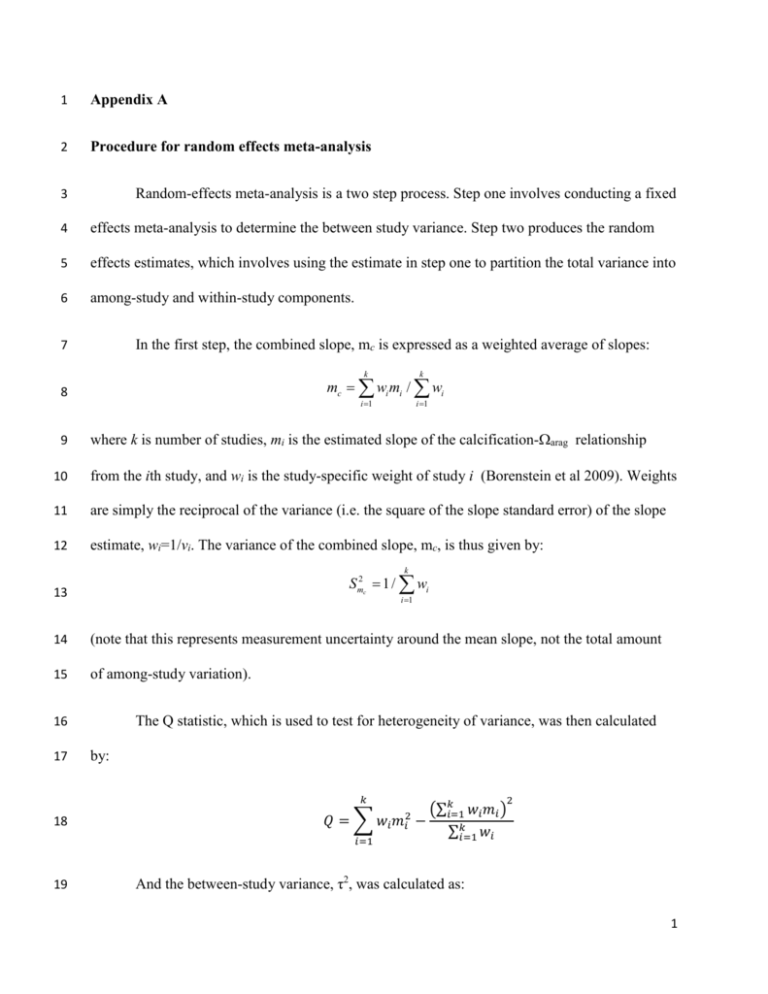
In the first step, the combined slope, mc is expressed as a weighted average of slopes:
8
9
k
k
i 1
i 1
mc   wi mi /  wi
where k is number of studies, mi is the estimated slope of the calcification-arag relationship
10
from the ith study, and wi is the study-specific weight of study i (Borenstein et al 2009). Weights
11
are simply the reciprocal of the variance (i.e. the square of the slope standard error) of the slope
12
estimate, wi=1/vi. The variance of the combined slope, mc, is thus given by:
k
S m2c  1/  wi
13
i 1
14
(note that this represents measurement uncertainty around the mean slope, not the total amount
15
of among-study variation).
16
17
The Q statistic, which is used to test for heterogeneity of variance, was then calculated
by:
𝑘
18
19
𝑄=
∑ 𝑤𝑖 𝑚𝑖2
𝑖=1
(∑𝑘𝑖=1 𝑤𝑖 𝑚𝑖 )
−
∑𝑘𝑖=1 𝑤𝑖
2
And the between-study variance, τ2, was calculated as:
1
𝑄 − 𝑑𝑓
𝑖𝑓 𝑄 > 𝑑𝑓
𝜏 ={ 𝐶
0
𝑖𝑓 𝑄 ≤ 𝑑𝑓
2
20
21
where C is a scaling factor to ensure that τ2 has the same units as the within-study variance, and
22
calculated by
23
∑ 𝑤𝑖2
𝐶 = ∑ 𝑤𝑖 −
∑𝑤
24
and df (degrees of freedom) is number of studies minus 1.
25
In the second step, the combined (within and between study) variance for each study is
𝑣𝑖∗ = 𝑣𝑖 + 𝜏 2
26
27
28
Combined slope, variance and 95% confidence intervals are then re-calculated as done in
step one but with the study weights wi* set equal to 1/𝑣𝑖∗ , instead of 1/𝑣𝑖 , as in step one.
29
30
31
32
Quantifying variance between studies
The I2 statistic, the ratio of excess dispersion to total dispersion, was calculated by
𝑸−𝒅𝒇
𝑰𝟐 = (
𝑸
) × 𝟏𝟎𝟎%
33
I2 values of 25%, 50% and 75% have been suggested as indicative of low, moderate and high
34
variance respectively (Higgins et al 2003).
35
Testing for between-group differences
36
The estimated difference between two effects is
2
𝜇𝐷𝑖𝑓𝑓 = 𝑀𝐵 − 𝑀𝐴
37
38
39
where MA & MB are the mean estimated slopes for groups A & B, calculated according to eq. 1
The standard error of this estimated difference is
𝜎𝐷𝑖𝑓𝑓 = √𝑉𝑀𝐴 + 𝑉𝑀𝐵
40
41
And thus the Z-statistic is
𝑍𝐷𝑖𝑓𝑓 =
42
43
𝜇𝐷𝑖𝑓𝑓
𝜎𝐷𝑖𝑓𝑓
Under the null hypothesis that the true mean effect size μ is the same for both groups
𝐻0 : 𝜇𝐴 = 𝜇𝐵
44
45
ZDiff would follow the normal distribution. For a two-tailed test the p-value is given by
46
𝑝 = 2 [1 − (𝛷(|𝑍𝐷𝑖𝑓𝑓 |))]
47
48
Meta-regression procedure
As with the original meta-analysis, meta-regression involves, first, a fixed effects meta-
49
regression to determine the between study variance, followed by a random effects step that
50
partitions the total variance into among-study and within-study components.
51
In step one, the fixed effects weighted regression uses the model:
52
𝑚𝑖 ~N(𝛼̂ + 𝛽̂ 𝑥𝑖 , 𝑣𝑖 )
3
53
Where mi is the estimated slope of the calcification-arag relationship from study i, xi is the value
54
of the explanatory variable (log(study duration) or log(irradiance level), depending on the meta-
55
regression) in study i, vi is the variance of the estimated slope within study i, 𝛽̂ represents the
56
change in the calcification-arag slope per unit change in the explanatory variable, and 𝛼̂ is the
57
intercept of the relationship between the calcification-arag slope, and the explanatory variable
58
(Thompson & Sharp 1999). N(𝛼̂ + 𝛽̂ 𝑥𝑖 , 𝑣𝑖 ) denotes a normal distribution with mean 𝛼̂ + 𝛽̂ 𝑥𝑖 and
59
variance 𝑣𝑖 . Maximum likelihood estimates of 𝛼̂ and 𝛽̂ were obtained by weighted least squares
60
regression (glm() in R) of mi on xi, with weights wi = 1/vi
The moment estimator of between-study variance, 𝜏 2 , was calculated as
61
𝜏2 =
62
63
64
65
66
67
68
𝑄−(𝑘−2)
𝐹(𝑤,𝑥)
if Q > k – 2, or 0 otherwise
where
𝑄 = ∑ 𝑤𝑖 (𝑦𝑖 − 𝛼̂ − 𝛽̂ 𝑥𝑖 )2
k is the number of studies, and
𝐹(𝑤, 𝑥) = ∑ 𝑤𝑖 −
∑ 𝑤𝑖2 ∑ 𝑤𝑖 𝑥𝑖2 −2 ∑ 𝑤𝑖2 𝑥𝑖 ∑ 𝑤𝑖 𝑥𝑖 +∑ 𝑤𝑖 ∑ 𝑤𝑖2 𝑥𝑖2
∑ 𝑤𝑖 ∑ 𝑤𝑖 𝑥𝑖2 −(∑ 𝑤𝑖 𝑥𝑖 )2
In step two, the random effects weighted regression uses the model
̂∗ 𝑥𝑖 , 𝑣𝑖∗ )
̂∗ + 𝛽
𝑚𝑖 ~𝑁(𝛼
69
̂∗ were obtained in the same way as 𝛼̂ and 𝛽̂ , except
̂∗ and 𝛽
Where vi*=vi+2, and estimates of 𝛼
70
with weights 𝑤𝑖∗ = 1/(𝑣𝑖 + 𝜏 2 ) used in place of 𝑤𝑖 = 1/𝑣𝑖 .
4
71
Publication Bias
72
The fail-safe number (X) is:
2
(∑ 𝑍𝑗 )
𝑋=
−𝐾
2.706
73
74
where Zj = Zrj√(Nj – 3), Zrj is Fisher’s z-transformed correlation coefficient for the relationship
75
between calcification and ΩAragonite for sample j, Nj is sample size for sample j and K is the
76
number of studies (Moller and Jennions 2001). The z-test value 2.706 (=1.6452) is based on a
77
one-tailed p value of 0.05 (Moller and Jennions 2001). Fisher’s z-transformed correlation
78
coefficient is:
1 1+𝑟
𝑍𝑟𝑗 = 𝑙𝑛
2 1−𝑟
79
80
where r is the correlation coefficient between calcification and ΩArag.
81
References
82
Borenstein M, Hedges LV, Higgins JPT, Rothstein HR (2009) Introduction to Meta-Analysis. John Wiley &
83
84
85
86
87
88
89
Sons, Hoboken, NJ, USA
Higgins J, Thompson SG, Deeks JJ, Altman DG (2003) Measuring inconsistency in meta-analysis. BMJ 327:
557-560
Moller AP, Jennions MD (2001) Testing and adjusting for publication bias. TRENDS in Ecology & Evolution
16: 580-586
Thompson SG, Sharp SJ (1999) Explaining heterogeneity in meta-analysis: A comparison of methods.
Statist. Med. 18: 2693-2708
90
5
91
92
93
94
6