Statistical modeling and machine learning for molecular biology
Alan Moses
Part I Statistical modelling
1. What is statistical modelling?
I think it’s important to make sure we are all starting at the same place. Therefore, before trying
to explain statistical modelling, I first want to discuss just plain modelling.
Modelling (for the purposes of this book) is the attempt to describe a series of measurements (or
other numbers or events) using mathematics. From the perspective of machine learning, a model
can only be considered useful if it can describe the series of measurements more succinctly (or
compactly) than the list of the numbers themselves. Indeed, in one particularly elegant
formulation, the information the machine “learns” is precisely the difference between the length
of the list of numbers and its compact representation in the model. However, another important
thing (in my opinion) to ask about a model besides its compactness is whether it provides some
kind of “insight” or “conceptual simplification” about the numbers in questions.
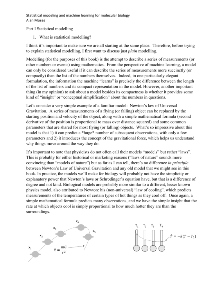
Let’s consider a very simple example of a familiar model: Newton’s law of Universal
Gravitation. A series of measurements of a flying (or falling) object can be replaced by the
starting position and velocity of the object, along with a simple mathematical formula (second
derivative of the position is proportional to mass over distance squared) and some common
parameters that are shared for most flying (or falling) objects. What’s so impressive about this
model is that 1) it can predict a *huge* number of subsequent observations, with only a few
parameters and 2) it introduces the concept of the gravitational force, which helps us understand
why things move around the way they do.
It’s important to note that physicists do not often call their models “models” but rather “laws”.
This is probably for either historical or marketing reasons (“laws of nature” sounds more
convincing than “models of nature”) but as far as I can tell, there’s no difference in principle
between Newton’s Law of Universal Gravitation and any old model that we might see in this
book. In practice, the models we’ll make for biology will probably not have the simplicity or
explanatory power that Newton’s laws or Schrodinger’s equation have, but that is a difference of
degree and not kind. Biological models are probably more similar to a different, lesser known
physics model, also attributed to Newton: his (non-universal) “law of cooling”, which predicts
measurements of the temperatures of certain types of hot things as they cool off. Once again, a
simple mathematical formula predicts many observations, and we have the simple insight that the
rate at which objects cool is simply proportional to how much hotter they are than the
surroundings.
x4
x3
x2
x1
T1
x5
T2
T3
T4
Statistical modeling and machine learning for molecular biology
Alan Moses
Figure 1 – example of observations and positions explained by Newton’s law of Universal
Gravitation and Newton’s law of cooling.
We now turn to statistical modelling, which is our point here. Statistical modelling also tries to
represent some observations of numbers or events – now called a “sample” or “data” – in a more
compact way, but it includes the possibility of randomness in the observations. Without getting
into a philosophical discussion of what this “randomness” is (see my next book) let’s just say
that statistical models acknowledge that the data will not be “fully” explained by the model.
Statistical models will be happy to predict something about the data, but they will not be able to
precisely reproduce the exact list of numbers. One might say, therefore, that statistical models
are inferior, because they don’t have the explaining power that, say, Newton’s laws have,
because Newton always gives you an exact answer. However, this assumes that you want to
explain your data exactly; in biology you almost never do. Every biologist knows that whenever
they write down a number, a part of the observation is actually just randomness or noise (or
inherent stochasticity?), due to methodological, biological or other experimental contingencies.
Indeed, it was a geneticist (Fisher) who really invented statistics after all -- 250 years after
Newton’s law of Universal Gravitation. Especially with the advent of high-throughput molecular
biology, it has never been more true that much of what we measure in biological experiments is
noise or randomness. We spend a lot of time and energy measuring things that we can’t and
don’t really want to explain. That’s why we need statistical modelling.
2. Probability distributions are the models
Luckily for Fisher, randomness had been studied for many years, because (it turns out) people
can get a big thrill out of random processes – dice and cards – especially if there’s money or
honour involved. Beautiful mathematical models of randomness can be applied to model the
part of biological data that can’t be (or isn’t interesting enough to be) explained. Importantly, in
so doing we will (hopefully) separate out the interesting part.
A very important concept in statistical modelling is that any set of data that we are considering
could be “independent and identically distributed” or “i.i.d” for short. I.i.d. means that all of the
measurements in the data set can be thought of as coming from the same “pool” of measurements
– so that the first observation could have just as easily been the seventh observation. In this
sense, the observations are identically distributed. Also, the observations don’t know or care
about what other observations have been made before (or will be made after) them. The eighth
coin toss is just as likely to come up “heads,” even if the first seven were also heads. In this
sense, the observations are independent. In general for data to be well-described by a simple
mathematical model, we will want our data to be i.i.d., and this assumption will be made
implicitly from now on, unless stated otherwise.
Statistical modeling and machine learning for molecular biology
Alan Moses
x1
x2
x3
x4 x5 x6
x6
x5
x4
x3
x2
x1
Figure 2 – observations in a pool, a Gaussian model for Fisher’s famous iris petal data. On top
right is the formula and the predicted “bell curve” for the Gaussian probability distribution.
As a first example of a statistical model, let’s consider the lengths of iris petals, very much like
what Fisher was thinking about while he was inventing statistics in the first place. Since iris
petals can be measured to arbitrary precision, we can treat these as so-called “real” numbers,
namely, numbers that can have decimal points or fractions, etc.
One favourite mathematical formula that we can use to describe the randomness of real numbers
is the Gaussian also called the Normal distribution, because it appears so ubiquitously that it is
simply “normal” to find real numbers with Gaussian distributions in nature.
More generally, this example shows that when we think about statistical modeling, we are not
trying to explain exactly what the observations will be: the iris petals are considered to be i.i.d.,
so if we measure another sample of petals, we will not observe the same numbers again. The
statistical model tries to say something useful about the sample of numbers, without trying to say
exactly what those numbers will be. The Gaussian distribution describes (quantitatively) the way
the numbers will tend to behave. This is the essence of statistical modelling.
Mathematical Box: deep thoughts about the Gaussian distribution.
The distribution was probably first introduced as an easier way to calculate binomial
probabilities, which were needed for predicting the outcome of dice games, which were very
popular even back in 1738. I do not find it obvious that there should be any mathematical
connection between predictions about of dice games and the shapes of iris petals. It is a quite
amazing fact of nature that the normal distribution describes both very well.
Another amazing thing about the Gaussian distribution is its strange formula. It’s surprising to
me that a distribution as ‘normal’ as the Gaussian would have such a strange looking formula.
Statistical modeling and machine learning for molecular biology
Alan Moses
Compare it too, say, the exponential distribution, which is just 𝑝(𝑥) = 𝜆𝑒 −𝜆𝑥 . The Gaussian
works because of a strange integral that relates the irrational number e, to another irrational
number pi.
∞
2
∫ 𝑒 −𝑥 𝑑𝑥 = √𝜋
−∞
This integral has a closed form solution only when taken from –infinity to +infinity.
Example Box: Models make assumptions and those assumptions have consequences.
For example, let’s consider data from a single cell RNA-seq experiment. For a given gene, we
probably have observed normalized numbers of reads. I took the measurements from 96 control
cells – these should be as close as we can get to i.i.d. The measurements we get are numbers
greater than or equal to 0, but many of them are exactly 0, so they aren’t well-described by a
Gaussian distribution. What about Poisson? This is a distribution that gives a probability to
seeing observations of exactly 0, but it’s really supposed to only model natural numbers like 0, 1,
2…, so it can’t actually predict probabilities for observations in between. The exponential is a
continuous distribution that is strictly positive, so it is another candidate for this data.
Attempts to fit this data with these standard distributions are shown in the figure. I hope it’s
clear that all of these models underpredict the large number of cells with low expression levels
(exactly 0) as well as the cells with very large expression levels. This example illustrates a
common problem in modelling genomic data. It doesn’t fit very well to any of the standard,
simplest models used in statistics. This motivates the use of fancier models, For example, the
data from single cell RNA-seq experiments can be modelled using a mixture model (which we
will meet in chapter 5).
Perhaps more important than the fit to the data is that the models make very different qualitative
claims about the data. For example, the Poisson model predicts that there’s a typical expression
level we expect (in this case around 4) and we don’t expect to see many cells with expression
levels much greater or less than that. On the other hand, the exponential model predicts that
many of the cells will have 0, and that the number of cells with expression above that will
decrease monotonically as the expression level gets larger. By choosing to describe our data
with one model or the other, we are making a very different decision about what’s important.
Number of cells
Statistical modeling and machine learning for molecular biology
Alan Moses
70
60
50
40
30
20
10
0
0 1 2
4 3 4 32
0
5 6 7 256
8 9
Interferon
Receptor 2 Series4
expression
Series3
(Reads per million)
Series2
Series1
Figure 3 – modelling single cell RNA-seq data from Shalek et al. The number of cells with each
expression level is shown with grey bars. The predictions of three probability distributions are
shown as lines and are indicated by their formulas: the exponential, Poisson and Gaussian
distributions are shown from top to bottom. The data was modelled in log space with 1 added to
each observation to avoid log(0), and parameters for each distribution were the Maximum
Likelihood estimates. The horizontal axis is a log scale.
This brings us to the first challenge that any researcher faces as they contemplate statistical
modelling and machine learning in molecular biology: what model (read: probability
distribution) should I choose for my data? Normal distributions (which I’ve said are the most
commonly found in nature) are defined for the real numbers, numbers like -6.72, 4.300, etc. If
you have numbers like this, consider yourself lucky because you might be able to use the
Gaussian distribution as your model. Molecular biology data comes in many different types, and
unfortunately much of it doesn’t follow a Gaussian distribution very well. Sometimes it’s
possible to transform the numbers to make the data a bit closer to Gaussian. The most common
way to do this is to try taking the logarithm. If your data are strictly positive numbers, this might
make the distribution more symmetric. And taking the logarithm will not change the relative
order of data points.
In molecular biology, there are 3 other major types of data that one typically encounters. First,
“Categorical” data describes data that is really not well-described by a sequence of numbers,
such as experiments that give “yes” or “no” answers, or molecular data, such as genome
sequences, that can be “A” “C” “G” or “T”. Second, “Fraction” or “Ratio” data is when the
observations are like a collection of yes or no answers, such as 13 out of 5212 or 73 As and 41
Cs. Finally, “ordinal” data is when data is drawn from the so-called “natural” numbers,
0,1,2,3,… In this case, it’s important that 2 is more than 1, but it’s not possible to observe
anything in between.
Depending on the data that the experiment produces, it will be necessary to choose appropriate
probability distributions to model it. In general you can test whether your data “fits” a certain
Statistical modeling and machine learning for molecular biology
Alan Moses
model by graphically comparing the distribution of the data to the distribution predicted by
statistical theory. A nice way to so this is using a quantile-quantile plot or ‘qq-plot’. This
compares the “theoretical quantiles” of a particular distribution to the quantiles in your data. If
they don’t disagree too badly, you can usually be safe assuming your data are consistent with
that distribution. It’s important to remember that with large genomics data sets, you will likely
have enough power to reject the hypothesis that your data “truly” come from any distribution.
Remember, there’s no reason that your experiment should generate data that follows some
mathematical formula. The observation that the data agrees at all with a mathematical formula is
the amazing thing.
Throughout this book, we will try to focus on techniques and methods that can be applied
regardless of the distribution chosen. Of course, in modern molecular biology we are often in the
situation where we produce data of more than one type, and we need a model that accounts for
multiple types of data. We will return to this issue in chapter 4.
3. Axioms of probability and their consequences: “rules of probability”
More generally, probability distributions are mathematical formulas that assign to events (or
more technically observations of events) numbers between 0 and 1. These numbers tell us
something about the relative rarity of the events. This bring us to my first “rule of probability” :
the sum of the probability of two observations is the probability of one or the other happening.
From this rule we can already infer another rule, which is that under a valid probability
distribution that the sum of all possible observations had better be exactly 1, because something
has to happen, but it’s not possible to observe more than one event in each try. (Although it’s a
bit confusing, observing “two” or “-7.62” of something would be considered one event for our
purposes here. We will soon consider probability distributions that model multiple simultaneous
events, known as multivariate distributions.)
The next important rule of probability is that the joint probability (the probability of a series of
independent events happening) is the product of the individual probabilities. The last and
possibly most important rule of probability is about conditional probabilities (probability of an
event given that another event already happened). The conditional probability is the joint
probability divided by the probability of the event that already happened.
Summary Box: Rules of Probability
1.
Probability of A or B is P(X=A) + P(Y=B), if X and Y are independent
2.
Sum of probabilities has to be 1. ∑𝐴,𝐵,𝐶… 𝑃(𝑋 = 𝐴) = 1
3.
Probability of A and B (aka. “joint” probability) P(X=A,Y=B) = P(X=A) P(Y=B), if X
and Y are independent
Statistical modeling and machine learning for molecular biology
Alan Moses
4.
Probability of A given B (aka. “conditional” probability) P(X=A|Y=B) =
P(X=A,Y=B)/P(Y=B)
Given these rules of probability, it’s now possible to understand Bayes’ Theorem:
𝑃(𝑋 = 𝐴|𝑌 = 𝐵) =
𝑃(𝑋 = 𝐴)
𝑃(𝑌 = 𝐵|𝑋 = 𝐴)
𝑃(𝑌 = 𝐵)
Bayes theorem is a key result that relates conditional probabilities. We’ll use it over and over
again in deriving statistical models. Another important idea that we’ll see in this book is the
expectation, which we denote as E[X] or <X>. You can think of this as our “best guess” about a
random variable, where you sum over all the possible values that the random variable can have,
weighting each by their probability.
𝐸[𝑋] = ∑ 𝑃(𝑋 = 𝐴)𝐴
𝐴,𝐵,𝐶…
An important thing to notice about the expectation is that it is a linear operator, so that E[X + Y]
= E[X] + E[Y] if X and Y are two random variables. Using the expectation operator it’s possible
to define the variance as V[X]=E[(X – E[X])2]
Box: notation and abuse of notation
I will do my best to use the simplest possible notations in this book, but in my efforts to do so, I
will have to leave out some details and write things that aren’t exact (or “abuse” the notation).
For example, you probably already noticed that I gave some formulas for probability
distributions as p(x), and now I’m using a new notation P(X=A). In the formula P(X=A), I’m
writing the probability that the random variable X takes the value A. Usually, I won’t both with
this and I’ll just write P(X) or p(X), and you’ll have to infer from context whether I’m talking
about the random variable or the value of the random variable. You’ll see that this is easier than
it sounds. I’ll be especially, loose with my use of the notation for conditional probabilities. I’ll
start writing probability distributions as p(X|parameters) or null distributions as p(X|H0 is true)
implying that the parameters or hypotheses are actually observations of random variables.
You might start thinking that it’s a bit strange to write models with parameters as random
variables, and that this assumption might cast philosophical doubt on the whole idea of
modelling as we discussed above. In practice, however, it’s easier not to think about it – we’re
using statistical models because they describe our data. We don’t really need to worry about
exactly what the notation means, as long as we’re happy with the predictions and data analysis
algorithms that we get.
4. Hypothesis testing – what you probably already know about statistics
So what about P-values? What I actually took away from my introductory statistics courses was
that somehow if an experiment was done properly, I could plug the numbers into a formula and it
would spit out a very small P-value, which meant the experiment “worked”. If the P-value
Statistical modeling and machine learning for molecular biology
Alan Moses
wasn’t that small, then the experiment didn’t work - that was bad, because it meant that you
probably had to do everything again.
P-values are the result of a “statistical hypothesis test.” For example, the t-test is specifically a
test of whether the mean of two lists of numbers are different. In “statistical hypothesis testing”
(the technical term for performing t-tests and other tests) the hypothesis that you are always
testing is the so-called “null hypothesis.” It’s very important to realize that the “null hypothesis”
that you are actually testing statistically is not usually the same as your actual (scientific)
hypothesis. In fact, it’s often exactly the opposite of the scientific hypothesis. In the case of the ttest, the null hypothesis is that the two lists of numbers truly have the same mean. Usually the
scientific hypothesis is that the two lists of numbers (e.g., describing mutant and wildtype) are
different.
Traditionally, hypothesis tests (such as the t-test) are generally set up in the following way.
Define a “test statistic” (some function of the data) whose distribution is known under the null
hypothesis, and look up the observed value of this test statistic in this so-called “null
distribution” to test the probability that the data were drawn from the null hypothesis. Since
finding a function of the data whose distribution was known (and possible to calculate by hand)
was very unusual, inventing these tests was a great achievement. Statistical tests were therefore
usually named after the distribution of the test statistic under the null hypothesis (the null
distribution) and/or after the statistician who discovered the test statistic (and sometimes a
combination of the two). So the null distribution for the (Student’s) t-test, is the Student’s tdistribution, because the test was proposed by a guy who called himself “Student” as a
pseudonym.
Using the “rules of probability” above, we can write all this a bit more formally:






H0, is the null hypothesis, which can be true or not.
The observations (or data) are X1, X2, … XN , which we will write as a vector X
t is a test statistic, t = f(X), where f represents some defined function.
the null distribution is therefore P( t | H0 is true)
t* is the observed value of the test statistic (for the set of data we have)
the P-value is P( t is “as or more extreme” than t* | H0 is true ), or P(t≥t*|H0) for short
Given these definitions, we also note that the distribution of P-values is also known under the
null hypothesis:

P(P-value < p | H0 is true) = p
In other words, under the null hypothesis, the P-value is a random variable that is uniformly
distributed between 0 and 1. This very useful property of P-values will come up in a variety of
settings. One example is “Fisher’s Method” for combining P-values. Given several different tests
with P-values p1, p2, …, pN you can combine them into a single P-value. Fisher figured out that
the test statistic 𝑡 = 𝑓(𝑝1 , 𝑝2 , … , 𝑝𝑁 ) = −2 ∑𝑖=𝑁
𝑖=1 ln(𝑝𝑖 ) is (approximately) chi-squared
distributed with 2N degrees of freedom if p1, p2, …, pN are uniformly distributed {0,1} and i.i.d.
0.25
0.3
0.05
0.25
0
0.2
0.15
0.1
Fraction of cells
0.15
0.35
0.1
0.2
0.2
0.15
0.15
Statistical
modeling and machine learning for molecular
0.35
0.15 biology 0.1
0.1
Alan Moses
0.3
0.1
0.05
0.05
This type of test (a test on the P-values of other tests) is also called “meta analysis” because you
0.25
0 the results of many analyses this0.05
can combine
way.
0
5 5.5 6 6.5 7 7.5 8 08.5 9 9.5 10
5 10.5
5.5 11
6 6.5 7 7.5 8 8.5 9
0.2
0.35
0.4
5 0.3 5.5 6 6.5 7 7.5 8 8.5 9 9.5 10
5 10.5
5.5 11
6 6.5 7 7.5 8 “ON”8.5
9 9.5 10 10.
0.35
Stem cells
cells
Series1
Series2
Series1
Series2
0.15
0.3
0.25
All
other
cells
0.25
“OFF”
cells
Series1
Series2
0.2
Series1
Series2
0.1
0.2
0.15
Fraction of cells
0.2
0.25
0.2
0.1
0.05
0.05
0.05
0
Fraction of cells
5
0
5.5
0.4
0.35
0.3
0.25
0.2
0.15
0.1
0.05
0
32
0.1
0.05
5 5.5 64
6 6.5 128
7 7.5 256
8 8.5 512
9 9.5 1024
10 10.5 11
32
0
0.15
0
5 5.5 64
6 6.5 128
7 7.5 256
8 8.5 512
9 9.5 1024
10 10.5 11
32
Series2
5Cdc6Series1
5.5
6 level6.5 7 7.5 8 8.5 9 9.5Theoretical
10Series1
10.5
11
expression
geneSeries2
expression
for a
normally distributed gene
6 6.5 7 7.5 8 T cells
8.5 9 9.5 10 10.5 11
Series1
Series2
All other cells
Series1
Series2
64
128
256
512
1024
2056
CD4 antigen expression level
Series1
Series2
Figure 4 – Testing hypotheses in practice with gene expression data from Immgen (refs). In each
plot the fraction of cells is plotted on the vertical axis as a function of the gene expression level
on the horizontal axis.
Take a real example. Stem cells are expected to be rapidly dividing, so we might expect them to
express genes involved in DNA replication, like Cdc6. Other cells, since they are differentiated
and not duplicating their DNA, might be expected to show no (or low) expression of DNA
replication genes like Cdc6. The null hypothesis is that Stem cells and other cells show the
same average Cdc6 expression level. Notice that this null hypothesis was actually the opposite of
our biological hypothesis. We can do a t-test (on the expression levels from Stem cells vs. the
expression levels from other cells) and calculate a P-value to test the hypothesis. In this case, the
t-statistic is -5.2979. If we look-up the probability of observing that t-statistic value or more in
the null distribution (the known distribution of the t-statistic given the null distribution is true,
which turns out to be a T-distribution), we get a P-value of 0.0001317. This means that the
chances of the Stem cells actually having the same average expression levels is very small,
which is great! This means that our data reject the null hypothesis, if the assumptions of the test
are true.
And this brings up the caveat to all P-value calculations – these P-values are only accurate as
long as the assumptions of the test are valid. Each statistical test has its own assumptions, and
this is just something that you always have to worry about when doing any kind of data analysis.
The t-test assumes that the data are normally distributed (but turns out to be reasonably robust to
violations of that assumption – the null distribution is still right when the data are only
approximately normally distributed). The t-test tests for differences in the mean. Consider the
data for CD4 antigen gene expression in Figure 3. Clearly the CD4 expression levels in T-cells
Statistical modeling and machine learning for molecular biology
Alan Moses
are more likely to be high in the T-cells than in the other cells, but the distribution is strongly bimodal – clearly not Gaussian. Although this probably does violate the assumptions of the t-test,
the more important issue is that only testing for a difference in the mean expression level is
probably not the best way to detect the difference.
5. Tests with fewer assumptions
In this context, and with the availability of computers and free statistics packages, it makes
practical sense to use tests with fewer assumptions. An important class of these tests are the socalled “non-parametric tests”. These are described in detail elsewhere, but we’ll review some
widely used examples to give the idea.
Wilcoxon-Rank-Sum test, also known as the Mann-Whitney U test (or simply the WMW-test)
The way the WMW test avoids “parameters” (assumptions about specific models or
distributions) by analysing only the relative ranks of the data, rather than the numerical values.
This is also a test that compares two lists of observations, to try to determine if one list tends to
have larger numbers than the other. To formulate the rank-based test, the data from the two lists
are combined, and the ranks are calculated based on the whole set. Then the ranks from the two
lists are added up separately and compared to the expected sum of the ranks for a list of numbers
that size. The expected sum of ranks can be calculated, and is just the number of observations
times the average rank. A little more formally,



The observations (or data) are X1, X2, … Xn and Y1, Y2, … Ym, which we will write as X
and Y
The ranks of the observations are R1, R2, … Rn+m, where each of the observations has
been assigned a rank in the entire dataset
There are two test statistics𝑈𝑋 =
𝑈𝑌 =
𝑛+𝑚+1
∑𝑖=𝑚
𝑖=1 𝑅𝑖 −𝑚
2
𝜎𝑈
𝑛+𝑚+1
2
∑𝑖=𝑛
𝑖=1 𝑅𝑖 −𝑛
𝜎𝑈
, based on the sum of the ranks of X, and
based on the sum of the ranks of Y.
In the formulas for the test statistic, the “average rank” shows up as
𝑛+𝑚+1
2
, so the expected sum
of ranks is just the average times the number of observations (n or m). You might recognize that
these test statistics have the form: observed average minus expected average divided by the
standard deviation. This type of standardized difference is often called a ‘Z-score.’ Amazingly,
the formula for the standard deviation of the ranks also has a reasonably simple formula, 𝜎𝑈 =
𝑚𝑛
√ 12 (𝑚 + 𝑛 + 1). However, it’s important to note that this formula assumes that there are no
tied ranks in the data. This means that you never saw the same number twice. In practice, you’ll
be using a statistics package to calculate these tests, so just make sure that the software is
handling the tied ranks properly.
Statistical modeling and machine learning for molecular biology
Alan Moses
Under the null hypothesis (that all the observations are drawn from a single distribution), these
test statistics turn out to be (approximately) Gaussian distributed, with mean and standard
deviation (0,1). The P-value for the WMW-test is the one associated with the U statistic that is
more extreme. Applying the WMW-test to the examples above, we get P=0.00008 for the Cdc6
data for Stem Cells, and P=0.00007 for the CD4 data.
Kolmogorov-Smirnov test (KS-test)
The KS-test is another example of a popular, rank-based test. Once again, the KS-test compares
two lists of numbers, under the null hypothesis that they are actually drawn from the same pool,
but this time it uses a test statistic based on the “cumulative distributions” of the observations.
The cumulative distribution is the sum of the probability0.35
distribution up to a certain point. The
0.35
KS-test uses as the test statistic the maximum difference between the cumulative distributions.
0.35
0.35 Figure 50.3
0.3 statistic, usually referred to as D.
illustrates the cumulative distribution and the KS-test
the distribution of this test statistic
(approximately) under the null
0.3 can be computed
0.3 Surprisingly,
0.25
0.25
hypothesis, regardless of the distribution of the data. I reproduce the formula here only for
0.25 aesthetic0.2
reasons – to show that there is no0.25
reason to expect
0.2that it should be simple:
0.2
0.2
0.15
∞
0.15
0.15−2𝑗 2 𝐷∗ 2 (0.12
𝑃(𝐷 < 𝐷∗ |𝐻0) ≈ 2 ∑(−1)𝑗−1 exp
0.1 +
0.1
0.15
0.1
[
𝑗=1
0.1
0.05
0.05
0.11
𝑛𝑚
𝑛+𝑚
𝑛𝑚 2
)
𝑛+𝑚
+√
√
]
Probability Density
Probability Density
is the exponential function, 0.05
D* is the observed0 value of the test statistic, and n and
0.05 Where exp[x]
0
m are the sizes of the two samples, as defined0in as in the WMW section.
5 10
5.5 10.5
6 11
6.5 7 7.5 8 8.5 9
5 5.5 6 6.5 7 7.5 8 8.5 9 9.5
0
5 5.5
6 11
6.5 7 7.5 8 T cells
8.5 9 9.5 10 10
0.6 10.5
5 0.45.5 6 6.5 7 7.5 8 T cells
8.5 9 9.5
10
Series1
Series2
0.35
Series1
Series2
0.5
0.3
Average
Series1
Series2
All other cells
0.4
Series1
Series2
0.25
Central Limit
0.2
0.15
0.1
0.05
0
Theorem
0.2
0.1
0
32
64
128
256
512
1024
2056
CD4 antigen expression level
Series1
Cumulative Distribution
0.3
32
64
128
256
512
1024
2056
CD4 antigen expression level
Series2
1.2
1
0.8
D
0.6
0.4
0.2
0
32
64
128
256
512
1024
2056
Series1
Series2
CD4 antigen
expression
level
Figure 5 – The KS-test and the central limit theorem apply even when the data are not distributed
according to a standard distribution.
Statistical modeling and machine learning for molecular biology
Alan Moses
Figure 5 illustrates why the KS-test would be expected to work reasonably well even on a
strongly bimodal dataset like the CD4 data. Like the WMW test, you will usually use a statistics
package to perform this test, and be sure that if there are any tied-ranks in your data, the statistics
software is handling them correctly. In the KS-test, it’s particularly tricky to handle the ties
correctly. Once again the KS-test tells us that both of these data sets are highly significant, with
the Cdc6 data having D = 0.6832, P = 1.038e-05, while the CD4 data have D = 0.3946, P =
5.925e-06. Notice that the Cdc6 data have a larger D, but are not as significant (large P-value).
This is because there are more T-cells than Stem Cells in the dataset. You can see the non-trivial
dependence on the size of the two sets in the formula for the KS-test P-value above.
6. Central Limit Theorem
The Central Limit Theorem is one of the least understood and most powerful results in statistics.
It explains at some deep level the connection between dice games and the shapes of Fisher’s iris
petals. The Central Limit Theorem can also help you devise statistical tests (or interpret data)
where the underlying observations are drawn from unknown or badly behaved distributions.
The key to understanding the central limit theorem is that it is about the distribution of means
(averages), not the observations themselves. The amazing result is that the distribution of the
means is known to be Gaussian, regardless of the distribution of underlying data, as long as they
have a finite mean and variance. A little more formally,



The observations (or sample) are X1, X2, … XN
1
𝐴(𝑋) = ∑𝑖=𝑁
𝑖=1 𝑋𝑖 , is just the ordinary average, which will give a different answer each
𝑁
time N data points are sampled from the pool.
If N is large enough, the distribution of A(X) will be a Gaussian, N(µ,σ2), where µ =
E[X], the true expectation of X, and variance σ2 = V[X]/N, the true variance of X divided
by the sample size.
This means that for samples of badly behaved (non-Gaussian) data, like the CD4 data shown in
the example, the distribution of averages will still be approximately Gaussian.
7. Exact tests and Gene Set Enrichment Analysis
Another important class of hypothesis tests that can be used to handle data with non-standard
distributions are related to Fisher’s exact test. These type of tests can be applied to continuous
data by first discretizing the data. For example, we can classify the CD4 data above into “high”
expression cells and “low” expression cells by choosing a cutoff. For example, if we say cells
with expression above 256 are “high” and cells with expression below 256 are “low” expression
cells, we can form the following two-by-two table:
T-cells
other cells
“high”
(>256)
24
17
“low”
(<256)
27
146
Statistical modeling and machine learning for molecular biology
Alan Moses
Note that there is a difference between the T-cells and the other cells: the T-cells are about 50%
“high” expression, and all the other cells are less than 20% “high” expression. We now need to
calculate the probability of having observed that big a difference in fraction (or ratio) under the
null hypothesis that the two groups is really have the same fraction (or ratio). A famous test for a
table like this is Pearson’s Chi-square test, which computes a test statistic based on the observed
and expected numbers in each cell. In Pearson’s test, however, the numbers in each cell have to
be “large enough” so that the approximation to the test statistic kicks in. Traditionally Pearson’s
test was used because it was easy to compute by hand, whereas Fisher’s Exact Test was difficult
(or impossible) to compute by hand. However, since we now use computers to do these tests, we
can always use Fisher’s exact test on this kind of data, which makes no assumptions about the
numbers in each cell.
Unlike traditional hypothesis tests, exact tests don’t really have a “test statistic” function that is
computed based on the data. Instead, Fisher’s test assigns a probability to every possible
configuration of numbers in the table under the null hypothesis that the numbers in each row and
column were randomly sampled from the total pool of observations (using a formula that I won’t
reproduce here.) To compute the P-value one adds up all the configurations with probability
smaller (more unlikely) than the observed configuration. Thus, the P-value is the probability of
observing a configuration as unlikely (or more unlikely) under the null hypothesis. Computing
this in practice requires a reasonably clever way to sum up the very large number of
configurations, and modern statistics packages might do this in various ways.
A similar exact test is used very often in the context of “Gene Set Enrichment Analysis.” In this
context, one has identified a list of genes in a molecular biology experiment (a gene set) and
wants to test whether the list of genes is random, or whether the experiment has identified genes
with specific biology associated (“enriched”). Initially, gene lists usually came from clustering of
gene expression data, often from microarrays. Gene set enrichment analysis was used to show
that genes with similar expression patterns with similarity measured in a high-dimensional space.
We will return to this type of data analysis in Chapter 5.
Now-a-days, Gene Set Enrichment Analysis is used on gene lists that arise from all types of data
analysis. For example, in 2012 we developed a new method to predict protein kinase-substrates
based on amino acid sequences, and wanted to know whether the set of predicted substrates
contained more previously known substrates than expected by chance. For example, we
predicted 46 Mec1 substrates, and of these 7 were already known to be substrates. Considering
there were only 30 known substrates in the databases, and we analyzed 4219 proteins in total, we
thought we were doing pretty well. A little more formally,

we have a sample, X1, X2, …, Xn , where each observation can either have a certain
property or not, which we denote as “positives” (Xi = 1) or “negatives” (Xi = 0).
Statistical modeling and machine learning for molecular biology
Alan Moses

The probability of observing the number positives 𝑘 = ∑𝑛𝑖=1 𝑋𝑖 if X was a random sample
from some finite pool, Y1, Y2, … Ym, with 𝑙 = ∑𝑚
𝑖=1 𝑌𝑖 positives total is given by the
hypergeometric distribution 𝑃𝐻𝑌𝑃 (𝑘|𝑛, 𝑙, 𝑚) =

(𝑘𝑙 )(𝑚−𝑙
𝑛−𝑘)
(𝑚
𝑛)
.
The P-value is
𝑖=min(𝑛,𝑙)
𝑃(≥ 𝑘|𝐻0) = ∑𝑖=𝑘
𝑖=𝑘−1
𝑃𝐻𝑌𝑃 ( 𝑖|𝑛, 𝑙, 𝑚) = 1 − ∑𝑖=0
𝑃𝐻𝑌𝑃 ( 𝑖|𝑛, 𝑙, 𝑚),
where the last equality 𝑃(≥ 𝑘|𝐻0) = 1 − 𝑃(< 𝑘|𝐻0) is just used to make the calculations
easier.
In practice, this type of exact test can usually only be calculated using a reasonably clever
𝑚!
statistics package, because to calculate (𝑚
) = 𝑛!(𝑚−𝑛)! in many examples requires computing
𝑛
very large factorials (e.g., 4219! = 1 x 2 x 3 x … x 4218 x 4219 is too large be stored as a
standard number on a computer).
8. Permutation tests
What if a situation arises where you have a hypothesis that isn’t summarized by any traditional
hypothesis test? For example, say you wanted to test if the mean is bigger and the standard
deviation is smaller. You might want to use the test statistic a(X) – sd(X) (where I used a() to
denote the mean and sd() for the standard deviation). Or maybe you think (for some reason) that
the ratio of the maximum to the average is what’s important in some condition. You might use
the test statistic max(X)/a(X). You might try figure out the distribution of your test statistic under
the null hypothesis, assuming you data were Gaussian.
However, another way to do it is to use your data to compute the null distribution explicitly using
a permutation test. These tests are particularly powerful when you are comparing two samples
(such as T-cells vs. other cells, or predicted “positives” vs. “negatives”). In all of these cases, the
null hypothesis is that the two samples are actually not different, or are drawn from the same
distribution. This means that it’s possible to construct an estimate of that distribution (the null
distribution) by putting the observations from the two sets into one pool, and then drawing
randomly the observations in the two samples. In the case of the CD4 measurements in T-cells
vs. other cells, we would mix all the T-cell measurements with the other cell measurements, and
then randomly draw a sample of the same size as the T-cell sample from the combined set of
measurements. Using this random, fake T-cell sample, we can go ahead and compute the test
statistic, just as we did on the real T-cell data. If we do this over and over again, we will obtain
many values for the test statistic. The distribution of the test statistic in these random samples is
exactly the null distribution to compare our test statistic to: these are the values of the test
statistic that we would have found if our T-cell sample was truly randomly drawn from the entire
set of measurements. If we sample enough times, eventually we will randomly pull the exact set
of values that are the real T-cell data, and get the exact value of the test statistic we observed. We
will also, on occasion, observe test statistics that exceed the value we observed in the real data.
Statistical modeling and machine learning for molecular biology
Alan Moses
Our estimate of the P-value is nothing more than the fraction of random samples where this
happens. This approach is sometimes referred to as “permuting the labels” because in some sense
we are forgetting the “label” (T-cell or not) when we create these random samples.
t
y y
x2 1x 3
x5 4
x3
x2 x5
x1 y2
t
x1 x3 y
x4 y1 3
x1 x2 x3 x x5 y1 y2 y3
4
t
Fraction of random samples
The great power of permutation tests is that you can get the null distribution for any test statistic
(or any function of the data) that you make up. Permutation tests also have several important
drawbacks: permutation tests involve large numbers of random samples from the data – this is
only possible with a computer, and if the number of samples needed is large or complicated, it
could take a very long time to get there. Probably more of an issue in practice is that for an
arbitrary test statistic, the permutation test needs to be “set up” by using some kind of
programmable statistics package. Finally, in order to implement a permutation test you have to
really understand your null hypothesis. This can become especially tricky if your data are
correlated or have complicated heterogeneity or structure.
0.3
0.25
t* observed in real data
0.2
0.15
P-value
0.1
0.05
0
-3 -2 -1 0 1 2 3 4 5 6 7 8
t
Figure 5 – illustration of how to obtain a P-value from permutation test. t indicates a test statistic,
which is just a function of a sample of numbers from the pool. By choosing random samples
from the pool according to the null hypothesis and computing the test statistic each time, you can
calculate the null distribution of the test statistic. To calculate the P-value, you sum up the area
under the null distribution that is more extreme than the value you observed for your real data.
Summary box: statistical tests
9. Some popular distributions.
Note that I won’t describe the distributions thoroughly here. All of this information is readily
available in much more detail on the internet or in standard statistics books. This section is really
for reference in later chapters. Although you won’t be able to memorize the formulas for these
distributions, you should try to remember the kinds of data that they can be used to model.
The Uniform distribution
This is the simplest of all distributions. It has a finite maximum and minimum, and assigns the
same probability to every number in the interval. So the probability of observing X is just
1/(maximum – minimum). Some people even use the word “random” to mean uniformly
distribution.
The T-distribution
Statistical modeling and machine learning for molecular biology
Alan Moses
You should think of the T-distribution as a “heavy tailed” approximation to a Gaussian
distribution with mean = 0 and standard deviation = 1. This means that it looks a lot like the
normal distribution, except that the probability in the tails of the distribution doesn’t decay as
fast as in the Gaussian. The similarity of the T-distribution to the Gaussian (with mean=0 and
standard deviation = 1) is controlled by the only parameter of the distribution, which is called the
“degrees of freedom” or df for short. When df=1 or 2 the tails of the T-distribution are quite a
bit heavier than the Gaussian. When df is around 30, the T-distribution starts to look a lot like a
Gaussian. Of course, only when df=infinity is the T-distribution *exactly* equal to the Gaussian
distribution.
The chi square distribution
The Exponential distribution
The Geometric distribution
The Poisson distribution
The Bernoulli distribution
The Binomial distribution
The Discrete or Categorical distribution
The Multinomial distribution
Summary Box: distributions
Excercises:
1. Derive Bayes’ Theorem
2. Show that Bayes’ Theorem is true even if the two events are independent.
3. Show that the geometric distribution is correctly normalized (i.e., the sum of all possible
1
𝑛
observations is 1) (hint: use the classical result that ∑∞
)
𝑛=0 𝑎 =
1−𝑎
4. It’s not quite true that –inf to inf is the only range for which the Gaussian integral can be
evaluated. There is one other range. What is it, and what’s the value of the integral?
(Hint: no calculations required – just think about the shape of the Gaussian distribution)
5. Explain why n + m + 1 divided by 2 is the expected average rank in the WMW test. (hint:
use the classical result that ∑𝑁
𝑗=1 𝑗 =
𝑁(𝑁+1)
2
)
6. Use the Central Limit Theorem to argue that the null distribution of the WMW test
statistic should be Gaussian
Statistical modeling and machine learning for molecular biology
Alan Moses
7. Consider the following two lists of numbers. The first list is 1,2, then ten 3s then 4 and 5.
The second list is the same, except there are one hundred 3s (instead of ten). Draw the
cumulative distributions for these two lists, and explain why this might lead to a problem
for the K-S test if ties were not handled correctly.
8. In the P-values for Gene Set Enrichment Analysis, why does the first sum go up only
until min(n,l) and the second one go up to k - 1?
References and further reading