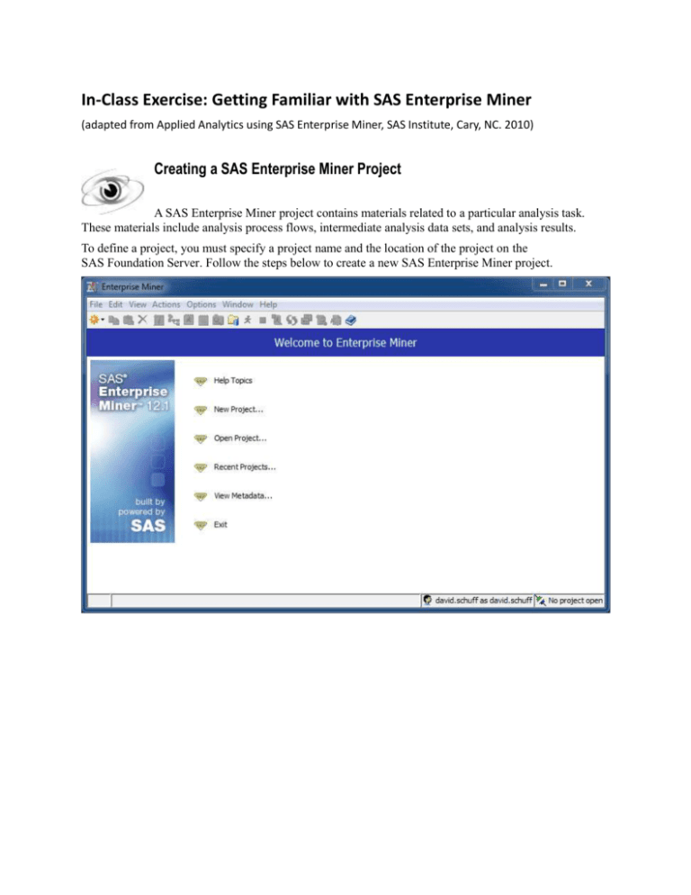
In-Class Exercise: Getting Familiar with SAS Enterprise Miner
(adapted from Applied Analytics using SAS Enterprise Miner, SAS Institute, Cary, NC. 2010)
Creating a SAS Enterprise Miner Project
A SAS Enterprise Miner project contains materials related to a particular analysis task.
These materials include analysis process flows, intermediate analysis data sets, and analysis results.
To define a project, you must specify a project name and the location of the project on the
SAS Foundation Server. Follow the steps below to create a new SAS Enterprise Miner project.
2
Getting Familiar with SAS Enterprise Miner
1. Select File  New  Project from the main menu. The Create New Project wizard opens at Step 1.
In this configuration of SAS Enterprise Miner, the only server available for processing is the host
server listed above.
2. Select Next >.
3. Name the project.
Step 2 of the Create New Project wizard is used to specify the following information:
 the name of the project you are creating
 the location of the project
3
4. Type a project name, for example, My Project, in the Name field.
The path specified by the SAS Server Directory field is the physical location where the
project folder will be created. This will look a little different for each account. That’s ok. Go with the
default.
5. Select Next >.

If you have an existing project directory with the same name and location as specified, this
project will be added to the list of available projects in SAS Enterprise Miner. This technique
can be used to import a project created by another installation of SAS Enterprise Miner.
6. Select a location for the project’s metadata.

The SAS folder, My Folder, is in a WebDAV directory. This is where the metadata associated
with the project is stored. This folder can be accessed and modified using SAS Management
Console.
4
Getting Familiar with SAS Enterprise Miner
7. Select Next >.
Information about your project is summarized in Step 4.
8. To finish defining the project, select Finish.
The SAS Enterprise Miner client application opens the project that you created.
5
Creating a SAS Enterprise Miner Diagram
A SAS Enterprise Miner diagram workspace contains and displays the steps involved in your analysis.
To define a diagram, you need only specify its name.
Follow the steps below to create a new SAS Enterprise Miner diagram workspace.
1. Select File  New  Diagram… from the main menu.
2. Type the name Predictive Analysis in the Diagram Name field and select OK.
SAS Enterprise Miner creates an analysis workspace window labeled Predictive Analysis.
You use the Predictive Analysis window to create process flow diagrams.
6
Getting Familiar with SAS Enterprise Miner
Defining a Data Sources
Specifying Source Data
A data source links SAS Enterprise Miner to a data table on the server. To specify a data source, you need
to define a SAS library and know the name of the table.
Follow these steps to specify a data source.
1. Select File  New  Data Source… from the main menu. The Data Source Wizard – Step 1 of 8
Metadata Source opens. The Data Source Wizard guides you through the process of creating a SAS
Enterprise Miner data source. Step 1 tells SAS Enterprise Miner where to find the right table.
Click on Source: and select Metadata Repository
2. Select Next >
The Data Source Wizard continues to Step 2 of 9 Select a SAS Table.
7
3. In this step, select the SAS table that you want to make available to SAS Enterprise Miner. Click
Browse on the right hand side.
4. Select the Shared Data  Libraries  AAEM  PVA97NK SAS table from the dialog.
5. Select OK. The Select a SAS Table window closes and the selected table appears in the Table field.
8
Getting Familiar with SAS Enterprise Miner
6. Select Next >. The Data Source Wizard proceeds to Step 3 of 8 (“Edit Library Allocation Code”).
Don’t make any changes here. Just click Next to go to the next screen (4 of 8 - “Table Information”).
This step of the Data Source Wizard provides basic information about the selected table.

The SAS table PVA97NK is used in this chapter and subsequent chapters to demonstrate the
predictive modeling tools of SAS Enterprise Miner. From this screen you can see the table
contains 9,686 cases and 28 variables.
Defining Column Metadata
With a data set specified, your next task is to set the column metadata. To do this, you need to know the
modeling role and proper measurement level of each variable in the source data set.
Follow these steps to define the column metadata:
1. Select Next >. The Data Source Wizard proceeds to Step 5 of 9 (Metadata Advisor Options).
s
9
This step of the Data Source Wizard starts the metadata definition process. This allows you to change
how SAS Enterprise Miner works with the data in the table. The Basic setting assigns initial values to
the metadata for each column in the table based on the variable name, data type, and assigned SAS
format. The Advanced setting assigns initial values to the metadata in the same way as the Basic
setting, but it also assesses the distribution of each variable to better determine the appropriate
measurement level.
2. Select Next > to use the Basic setting.
The Data Source Wizard proceeds to Step 6 of 9, Column Metadata.
The Data Source Wizard displays SAS’ best guess for the metadata assignments. The correct values
for model role and measurement level are found in the PVA97NK metadata table on the next page.
A comparison with the metadata table on the next page shows several discrepancies. While the
assigned modeling roles are mostly correct, the assigned measurement levels for several variables
need to be fixed – they’re not the way we want them for the analysis.
10
Getting Familiar with SAS Enterprise Miner
It is possible to improve the default metadata assignments by using the Advanced option in the
Metadata Advisor.
3. Select < Back in the Data Source Wizard. This returns you to Step 5 of 9 Metadata Advisor Options.
4. Select the Advanced option. Then select Next >.
PVA97NK Metadata Table
Model
Role
Name
Measurement
Level
Description
DemAge
Input
Interval
Age
DemCluster
Input
Nominal
Demographic Cluster
DemGender
Input
Nominal
Gender
DemHomeOwner
Input
Binary
Home Owner
DemMedHomeValue
Input
Interval
Median Home Value Region
DemMedIncome
Input
Interval
Median Income Region
DemPctVeterans
Input
Interval
Percent Veterans Region
GiftAvg36
Input
Interval
Gift Amount Average 36 Months
GiftAvgAll
Input
Interval
Gift Amount Average All Months
GiftAvgCard36
Input
Interval
Gift Amount Average Card 36 Months
GiftAvgLast
Input
Interval
Gift Amount Last
GiftCnt36
Input
Interval
Gift Count 36 Months
GiftCntAll
Input
Interval
Gift Count All Months
GiftCntCard36
Input
Interval
Gift Count Card 36 Months
GiftCntCardAll
Input
Interval
Gift Count Card All Months
GiftTimeFirst
Input
Interval
Time Since First Gift
GiftTimeLast
Input
Interval
Time Since Last Gift
ID
ID
Nominal
Control Number
PromCnt12
Input
Interval
Promotion Count 12 Months
PromCnt36
Input
Interval
Promotion Count 36 Months
PromCntAll
Input
Interval
Promotion Count All Months
PromCntCard12
Input
Interval
Promotion Count Card 12 Months
PromCntCard36
Input
Interval
Promotion Count Card 36 Months
PromCntCardAll
Input
Interval
Promotion Count Card All Months
StatusCat96NK
Input
Nominal
Status Category 96NK
StatusCatStarAll
Input
Binary
Status Category Star All Months
TargetB
Target
Binary
Target Gift Flag
TargetD
Rejected
Interval
Target Gift Amount
11
5. The Data Source Wizard again proceeds to Step 6 of 9 “Column Metadata.”
s
While many of the default metadata settings are correct, there are still several items that need to be
changed. For example, the DemCluster variable is rejected (for having too many distinct values),
and several numeric inputs have their measurement level set to Nominal instead of Interval (for
having too few distinct values).
(By the way, “Nominal” means that the order of the values is not meaningful – i.e., say 1 is female
and 2 is male – these are categorizations but it’s not that 2 is “greater” or “less” than 1. “Interval”
means it’s a continuous variable – the values are on an equally spaced scale and not distinct
categorizations. Height and weight are examples of interval variables – the difference between 5
pounds and 10 pounds is the same as the difference between 10 pounds and 15 pounds.
To avoid the time-consuming task of making metadata adjustments, go back to the previous Data
Source Wizard step and customize the Metadata Advisor.
6. Select < Back. You return to the Metadata Advisor Options window.
12
Getting Familiar with SAS Enterprise Miner
7. Select Customize…. The Advanced Advisor Options dialog box opens.
Using the default Advanced options, the Metadata Advisor can do the following:
 reject variables with an excessive number of missing values (default=50%)

detect the number class levels of numeric variables and assign a role of Nominal to those with
class counts below the selected threshold (default=20)

detect the number class levels of character variables and assign a role of Rejected to those
with class counts above the selected threshold (default=20)

In the PVA97NK table, there are several numeric variables with fewer than 20 distinct values
that should not be treated as nominal. Similarly, there is one class variable with more than 20
levels that should not be rejected.
To avoid changing many metadata values in the next step of the Data Source Wizard, you
should alter these defaults.
8. Change the value for the Class Levels Count Threshold value to 3. This ensures that only binary
variables are treated as categorical (i.e., anything with LESS than 3 values – i.e., 0 and 1).
9. Also type 100 as the Reject Levels Count Threshold value, so that only character variables with more
than 100 distinct values are rejected.
 Be sure to press ENTER after you type the number 100. Otherwise, the value might not be
registered in the field.
Your dialog should look like this:
13
10. Select OK to close the Advanced Advisor Options dialog box.
11. Select Next > to proceed to Step 6 of 9 in the Data Source Wizard.
14
Getting Familiar with SAS Enterprise Miner
A comparison of the Column Metadata table to the table at the beginning of the demonstration shows
that now most of the metadata is correctly defined. SAS Enterprise Miner correctly inferred the model
roles for the non-input variables by their names. The measurement levels are correctly defined by
using the Advanced Metadata Advisor.
The analysis of the PVA97NK data in this course focuses on the TargetB variable, so the TargetD
variable should be rejected.
12. Select Role  Rejected for TargetD.
In summary, Step 6 of 9 (Column Metadata) is usually the most time-consuming of the Data Source
Wizard steps. You can use the following tips to reduce the amount of time required to define metadata
for SAS Enterprise Miner predictive modeling data sets:
 Only include variables that you intend to use in the modeling process in your raw data source.
 For variables that are not inputs, use variable names that start with the intended role. For example,
an ID variable should start with ID and a target variable should start with Target.
 Inputs that are to have a nominal measurement level should have a character data type.
 Inputs that are to be interval must have a numeric data type.
 Customize the Metadata Advisor to have a Class Level Count set equal to 3 and a Reject Levels
Count set equal to a number greater than the maximum level count of your nominal inputs.
Finalizing the Data Source Specification
Follow these steps to complete the data source specification process:
1. Select Next > to proceed to Decision Configuration. We don’t need to configure this – the data set is
already set up to work with the predictive modeling techniques we’re going to do. So just select No
and then select Next >.
15
2. You will be asked whether you want to create a sample data set (Step 8 of 10). Make sure “No” is
selected and click Next> again.
3. Now you’ll reach step 9 of 10 in the Data Source Wizard.
This step enables you to set a role for the data source and add descriptive comments about the data
source definition. For the upcoming analysis, a table role of Raw is acceptable.
4. The final step in the Data Source Wizard provides summary details about the data table that you
created. Select Finish.
16
Getting Familiar with SAS Enterprise Miner
5. The PVA97NK data source is added to the Data Sources entry in the Project panel.
6. You can view the properties of the PVA97NK data source by clicking once on the name of that data
source (listed under “Data Sources”).
17
Exploring Source Data
SAS Enterprise Miner can construct interactive plots to help you explore your data. This demonstration
shows the basic features of the Explore window. These include the following:
 opening the Explore window
 changing the Explore window sample size
 creating a histogram for a single variable
 changing graph properties for a histogram
 changing chart axes
 adding a missing bin to a histogram
 adding plots to the Explore window
 exploring variable associations
18
Getting Familiar with SAS Enterprise Miner
Opening the Explore Window
There are several ways to access the Explore window. Use these steps to open the Explore window
through the Project panel.
1. Make sure the Data Sources folder in the Project panel is open and right-click the data source
PVA97NK. The Data Source Option menu appears. Select Explore…
It will take a few seconds for the next window to open. It’s reading the entire data set.
19
2. Now you’ll see information about the data set:
The Explore window features a 2000-observation sample from the PVA97NK data source. Sample
properties are shown in the top half of the window and a data table is shown in the bottom half.
3. If at first you cannot see any tables here, select Window  Tile. The windows should then become
visible.
20
Getting Familiar with SAS Enterprise Miner
Changing the Explore Sample Size
The Sample Method property indicates that the sample is drawn from the top (first 2000 rows) of the data
set. Use these steps to change the sampling properties in the Explore window.

Although selecting a sample through this method is quick to execute, fetching the top rows of a
table might not produce a representative sample of the table.
1. Left-click the Sample Method value field. The Option menu lists two choices: Top (the current
setting) and Random.
2. Select Random from the drop-down list.
3. Select Actions  Apply Sample Properties from the Explore window menu. A new, random sample
of 2000 observations is made. This 2000-row sample now has distributional properties that are similar
to the original 9686 observation table. This gives you an idea about the general characteristics of the
variables. If your goal is to examine the data for potential problems, it is wise to examine the entire
data set.

SAS Enterprise Miner enables you to increase the sample transferred to the client (up to a
maximum of 30,000 observations). See the SAS Enterprise Miner Help file to learn how to
increase this maximum value.
4. Select the Fetch Size property and select Max from the Option menu.
5. Select Actions  Apply Sample Properties. Because there are fewer than 30,000 observations, the
entire PVA97NK table is transferred to the SAS Enterprise Miner client machine, as indicated by the
Fetched Rows field.
21
Creating a Histogram for a Single Variable
While you can use the Explore window to browse a data set, its primary purpose is to create statistical
analysis plots. Use these steps to create a histogram in the Explore window.
1. Select Actions  Plot from the Explore window menu. The Chart wizard opens to the Select a Chart
Type step. The Chart wizard enables the construction of a multitude of analysis charts. This
demonstration focuses on histograms.
2. Select Histogram.
Histograms are useful for exploring the distribution of values in a variable.
3. Select Next >. The Chart wizard proceeds to the next step, Select Chart Roles.
To draw a histogram, one variable must be selected to have the role X.
4. Select Role  X for the DEMAGE variable.
Then click Next...
22
Getting Familiar with SAS Enterprise Miner
5. You will then be presented with a window asking if you want to filter the data plotted in the
histogram based on some WHERE condition. We don’t need to do this now, so click Finish.
6. You will see the histogram of the DEMAGE variable.

Variable descriptions, rather than variable names, are used to label the axes of plots.
Axes in Explore window plots are chosen to range from the minimum to the maximum values of the
plotted variable. Here you can see that Age has a minimum value of 0 and a maximum value of 87.
The mode occurs in the ninth bin, which ranges between about 70 and 78. Frequency tells you that
there are about 1400 observations in this range.
Changing the Graph Properties for a Histogram
By default, a histogram in SAS Enterprise Miner has 10 bins and is scaled to show the entire range of
data. Use these steps to change the number of bins in a histogram and change the range of the axes.
While the default bin size is sufficient to show the general shape of a variable’s distribution, it is
sometimes useful to increase the number of bins to improve the histogram’s resolution.
1. Right-click in the data area of the Age histogram and select Graph Properties… from the Option
menu. The Properties-Histogram window opens.
This window enables you to change the appearance of your charts. For histograms, the most
important appearance property (at least in a statistical sense) is the number of bins.
23
2. Type 87 into the Number of X Bins field.
Because Age is integer-valued and the original distribution plot had a maximum of 87, there will be
one bin per possible Age value.
24
Getting Familiar with SAS Enterprise Miner
3. Select OK. The Explore window reopens and shows many more bins in the Age histogram.
With the increase in resolution, unusual features become apparent in the Age variable. For example,
there are unexpected spikes in the histogram at 10-year intervals, starting at Age=7. Also, you must
question the veracity of ages below 18 for donors to the charity.
25
Adding Plots to the Explore Window
You can add other plots to the Explore window. Follow these steps to add a pie chart of the target
variable.
1. Select Actions  Plot from the Explore window menu. The Chart wizard opens to the Select a Chart
Type step.
2. Scroll down in the chart list and select a Pie chart.
3. Select Next >. The Chart wizard continues to the Select Chart Roles step.
The message at the top of the Select Chart Roles window states that a variable must be assigned the
Category role.
4. Scroll the variable list and select Role  Category for the TARGETB variable. Again, skip over the
data filtering option and click Finish.
26
Getting Familiar with SAS Enterprise Miner
5. Select Finish to create the pie chart for TARGETB.
s
The chart shows an equal number of cases for TARGETB=0 (top) and TARGETB=1 (bottom).
27
6. Select Window  Tile to simultaneously view all sub-windows of the Explore window.
28
Getting Familiar with SAS Enterprise Miner
Exploring Variable Associations
All elements of the Explore window are connected. By selecting a bar in one histogram, for example,
corresponding observations in the data table and other plots are also selected. Follow these steps to use
this feature to explore variable associations:
1. Double-click the Age histogram title bar so that it fills the Explore window.
2. Click and drag a rectangle in the Age histogram to select cases with Age in excess of 70 years.
The selected cases are cross-hatched. (The vertical axis is rescaled to show the selection more
clearly.)
29
3. Double-click the histogram title bar again. The display is restored.
Notice that part of the TargetB pie chart is selected. This selection shows the relative proportion of
observations with Age greater than 70 that do and do not donate. Because the arc on the TARGETB=1
segment is slightly thicker, it appears that there is a slightly higher number of donors than non-donors
in this Age selection.
4. Close the Explore window to return to the SAS Enterprise Miner client interface screen.
30
Getting Familiar with SAS Enterprise Miner
Changing the Explore Window Sampling Defaults
Follow these steps to change the SAS Enterprise Miner preferences to use a random sample
for all of the data source data in the Explore window:
NOTE: This is very important. If you don’t do these next steps correctly you
will get the wrong answers for future in-class exercises and assignments!!
1. Select Options  Preferences… from the main menu. The Preferences window will open.
2. Select Sample Method  Random and select Fetch Size  Max.
With these settings, the Explore window uses the entire data set or a random sample of up to 30,000
observations (whichever is smaller).
3. Click OK.
31
Modifying and Correcting Source Data
This demonstration shows you how to replace a placeholder value for missing with a true missing value
indicator. In this way, SAS Enterprise Miner tools can correctly respond to the true, but unknown, value.
SAS Enterprise Miner includes several tools that you can use to modify the source data for your analysis.
First, create a histogram for the DemMedIncome variable. You’ve done these steps before, so
1. Right-click on the PVA97NK data source and select Explore…
2. The Explore window will appear. Select Actions/Plot…
3. Select Histogram and click Next…
4. Give the DemMedIncome variable the Role of “X”
32
Getting Familiar with SAS Enterprise Miner
5. Click the Finish button and you’ll see the histogram:
6. Right-click anywhere inside the chart area and select Graph Properties…
7. Change the number of X Bins to 50 and click the OK button. You’ll now see the following:
33
This reveals that the original appearance of a high number (frequency) of people with an income between
$0 and $20,000 actually is misleading. In reality, there is an unusual spike at 0.
This phenomenon often occurs in data extracted from a relational database table where 0 or another
number is used as a substitute for the value that is missing or unknown.
The distinction is very important – having zero income is very different from having an “unknown”
income. If you properly use the income variable in a predictive model, this discrepancy can be
addressed.
The following demonstrations show how to use the Replacement node to modify incorrect or improper
values for a variable.
Process Flow Setup
Use the following steps to set up the process flow that will modify the DemMedIncome variable:
1. Make sure you close the window with the histogram. You need to get back to the main Enterprise
Miner screen.
2. Drag the PVA97NK data source to the Predictive Analysis workspace window.
34
Getting Familiar with SAS Enterprise Miner
3. Select the Modify tab to access the Modify tool group. Drag the Replacement tool (third from the
right) from the Tools Palette into the Predictive Analysis workspace window.
4. Connect the PVA97NK data to the Replacement node by clicking near the right side of the PVA97NK
node and dragging an arrow (it will look like you’re drawing with a pencil on the screen) to the left
side of the Replacement node.
You created a process flow, which is the method that SAS Enterprise Miner uses to carry out
analyses. This process flow reads the PVA97NK data and replaces the unwanted values of the
observations. You must, however, specify which variables have unwanted values and what the correct
values are. To do this, you must change the settings of the Replacement node.
35
Changing the Replacement Node Properties
Use the following steps to modify the default settings of the Replacement node:
1. Select the Replacement node and examine the Properties panel.
The Properties panel displays the analysis methods used by the node when it is run. By default, the
node replaces all interval variables whose values are more than three standard deviations from the
variable mean.

You can control the number of standard deviations by selecting the Cutoff Values property.
In this demonstration, you only want to replace the value for DemMedIncome when it equals zero.
Thus, you need to change the default setting.
2. Select the Default Limits Method property and select None from the Options menu.
You want to replace improper values with missing values. To do this, you need to change the
Replacement Value property.
36
Getting Familiar with SAS Enterprise Miner
3. Select the Replacement Values property and select Missing from the Options menu.
You are now ready to specify the variables that you want to replace.
4. Select the ellipsis
(look under Interval Variables/Replacement Editor under the Train section) from
the properties panel.

Be careful to open the Replacement Editor for Interval Variables, not for Class Variables.
37
The Interactive Replacement Interval Filter window opens.
s
5. Select User Specified as the Limit Method value for DemMedIncome.
38
Getting Familiar with SAS Enterprise Miner
6. Type 1.0 as the Lower Limit value for DemMedIncome. It will appear as 1.
If you use this specification, any DemMedIncome values that fall below the lower limit of 1 are set
to missing. All other values of this variable do not change.
7. Select OK to close the Interactive Replacement Interval Filter window.
39
Running the Analysis and Viewing the Results
Use these steps to run the process flow that you created.
1. Right-click on the Replacement node and select Run from the Option menu. A Confirmation
window appears, and requests that you verify the run action.
2. Select Yes to close the Confirmation window. A small animation in the lower right corner of each
node indicates analysis activity in the node.
The Run Status window opens when the process flow run is complete.
3. Select Results… to review the analysis outcome. The Results - Node: Replacement Diagram:
Predictive Analysis window appears.
40
Getting Familiar with SAS Enterprise Miner
The Replacement Counts window shows that 2357 observations were modified by the Replacement
node. The Interval Variables window summarizes the replacement that was conducted. The Output
window provides more or less the same information as the Total Replacement Counts window and the
Interval Variables window (but it is presented as a static text file).
4. Close the Results window.