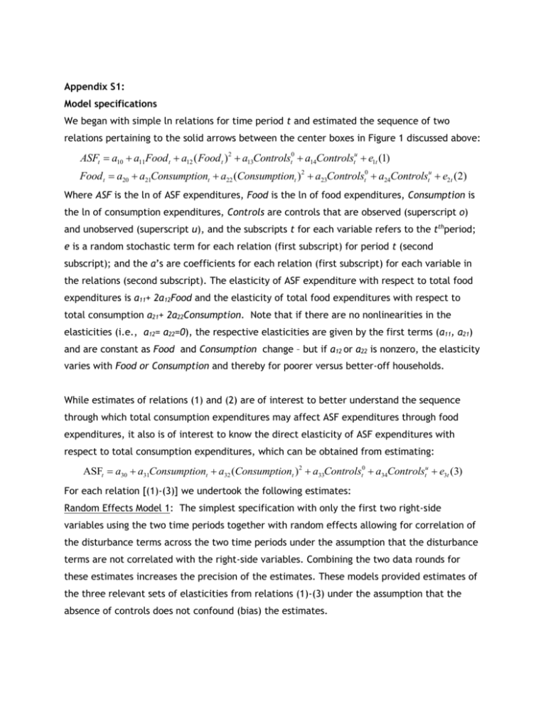
Appendix S1:
Model specifications
We began with simple ln relations for time period t and estimated the sequence of two
relations pertaining to the solid arrows between the center boxes in Figure 1 discussed above:
ASFt  a10  a11Food t  a12 ( Food t )2  a13Controlst0  a14Controlstu  e1t (1)
Food t  a20  a21Consumptiont  a22 (Consumptiont )2  a23Controlst0  a24Controlstu  e2 t (2)
Where ASF is the ln of ASF expenditures, Food is the ln of food expenditures, Consumption is
the ln of consumption expenditures, Controls are controls that are observed (superscript o)
and unobserved (superscript u), and the subscripts t for each variable refers to the tthperiod;
e is a random stochastic term for each relation (first subscript) for period t (second
subscript); and the a’s are coefficients for each relation (first subscript) for each variable in
the relations (second subscript). The elasticity of ASF expenditure with respect to total food
expenditures is a11+ 2a12Food and the elasticity of total food expenditures with respect to
total consumption a21+ 2a22Consumption. Note that if there are no nonlinearities in the
elasticities (i.e., a12= a22=0), the respective elasticities are given by the first terms (a11, a21)
and are constant as Food and Consumption change – but if a12 or a22 is nonzero, the elasticity
varies with Food or Consumption and thereby for poorer versus better-off households.
While estimates of relations (1) and (2) are of interest to better understand the sequence
through which total consumption expenditures may affect ASF expenditures through food
expenditures, it also is of interest to know the direct elasticity of ASF expenditures with
respect to total consumption expenditures, which can be obtained from estimating:
ASFt  a30  a31Consumptiont  a32 (Consumptiont ) 2  a33Controlst0  a34Controlstu  e3t (3)
For each relation [(1)-(3)] we undertook the following estimates:
Random Effects Model 1: The simplest specification with only the first two right-side
variables using the two time periods together with random effects allowing for correlation of
the disturbance terms across the two time periods under the assumption that the disturbance
terms are not correlated with the right-side variables. Combining the two data rounds for
these estimates increases the precision of the estimates. These models provided estimates of
the three relevant sets of elasticities from relations (1)-(3) under the assumption that the
absence of controls does not confound (bias) the estimates.
Random Effects with Controls Model 2: Model 1 plus standard observed controls (parental
schooling, community wealth). These provided insight into whether the absence of observed
controls biased the simple estimates and altered the estimated elasticities with such controls,
all under the assumption that the absence of controls for the unobserved variables did not
confound (bias) the estimates.
Fixed Effects Model 3: Model 3 with household fixed effects to control for unobserved fixed
controls (e.g., some households may have preferences that lead to higher material wealth
and consumption and to more ASF, so failure to control for such preferences biases upwards
the consumption coefficient estimates), common unobserved trends shared experienced by all
households (that, if not controlled and if correlated with the right-side expenditure variables
also result may cause biases in the elasticities of the expenditure variables of interest) and
for observed fixed controls (such as head and spouse education) to see if these estimates
were preferred to the random effects estimates without control for the unobserved fixed
effects and common unobserved trends and to see whether the elasticities of interest were
affected by controlling for the unobserved fixed effects and common trends. We reported
Hausman’s p that tests whether the fixed effects models are preferred over the random
effects models. Based on the estimates of the multivariate relations, we estimated
elasticities of ASF expenditures under multiple scenarios.