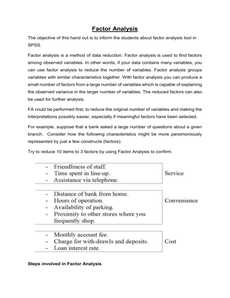
Factor Analysis
The objective of this hand out is to inform the students about factor analysis tool in
SPSS.
Factor analysis is a method of data reduction. Factor analysis is used to find factors
among observed variables. In other words, if your data contains many variables, you
can use factor analysis to reduce the number of variables. Factor analysis groups
variables with similar characteristics together. With factor analysis you can produce a
small number of factors from a large number of variables which is capable of explaining
the observed variance in the larger number of variables. The reduced factors can also
be used for further analysis.
FA could be performed first, to reduce the original number of variables and making the
interpretations possibly easier, especially if meaningful factors have been selected.
For example, suppose that a bank asked a large number of questions about a given
branch. Consider how the following characteristics might be more parsimoniously
represented by just a few constructs (factors).
Try to reduce 10 items to 3 factors by using Factor Analysis to confirm.
Steps involved in Factor Analysis
1. First, a correlation matrix is generated for all the variables. A correlation matrix is a
rectangular array of the correlation coefficients of the variables with each other.
2. Second, factors are extracted from the correlation matrix based on the correlation
coefficients of the variables.
3. Third, the factors are rotated in order to maximize the relationship between the
variables and some of the factors.
Task 1: Running the Factor Analysis Procedure
From the menu bar select Analyze and choose Data Reduction and then click on
Factor. Highlight related variables and send them to variables lists. Then select some
options and run the procedure.
The Factor Analysis dialogue box
Click on the DESCRIPTIVES button and its dialogue box will be loaded on the screen.
Within this dialogue box select the following check boxes Univariate Descriptives,
Coefficients, Determinant, KMO and Bartlett's test of sphericity, and
Reproduced. Click on Continue to return to the Factor Analysis dialogue box.
The Factor Analysis: Descriptive dialogue box should be completed as shown below.
From the Factor Analysis dialogue box click on the EXTRACTION button and its
dialogue box will be loaded on the screen. Select the check box for Scree Plot. Click
on Continue to return to the Factor Analysis dialogue box. The Factor Analysis:
Extraction dialogue box should be completed as shown below.
The Factor Analysis: Extraction dialogue box
From the Factor Analysis dialogue box click on the ROTATION button and its dialogue
box will be loaded on the screen. Click on the radio button next to Varimax to select
it. Click on Continue to return to the Factor Analysis dialogue box. The Factor
Analysis: Rotation dialogue box should be completed as shown below.
The Factor Analysis: Rotation dialogue box
From the Factor Analysis dialogue box click on the OPTIONS button and its dialogue
box will be loaded on the screen. Click on the check box of Suppress absolute values
less than to select it. Type 0.50 in the text box. Click on Continue to return to the
Factor Analysis dialogue box. Click on OK to run the procedure. The Factor Analysis:
Options dialogue box should be completed as shown below.
The Factor Analysis: Options dialogue box
Now you will be able to see the results of factor analysis and we could interpret the
results.
Let’s do an example for understanding factor analysis.
Following figure will show the SPSS data used in this analysis
.
After doing the Factor analysis procedures mentioned above, you will get the following
output.
Let us look at the first output,
This table shows you the actual factors that were extracted. If you look at the section
labelled “Rotation Sums of Squared Loadings,” it shows you only those factors that
met your cut-off criterion (extraction method). In this case, there were three factors
with eigenvalues greater than 1.
SPSS always extracts as many factors initially as there are variables in the dataset,
but the rest of these didn’t make the grade. The “% of variance” column tells you how
much of the total variability (in all of the variables together) can be accounted for by
each of these summary scales or factors. Factor 1 accounts for 34.88% of the
variability in all 13 variables, Factor 2 accounts for 19.33% of the variability in all 13
variables and Factor 3 accounts for 15.6% of the variability in all 13 variables so on.
We can see that altogether these three factors accounted for the 69.8% of total
variance.
Let us look at the second table
Finally, the Rotated Component Matrix shows you the factor loadings for each
variable. I went across each row, and highlighted the factor that each variable loaded
most strongly on. Based on these factor loadings, we know exactly which items belong to
factor1, 2, and 3.
Factor 1
Expensive
Factor 2
Factor 3
Appeals to Others
Reliable
Attractive Looking
Latest Features
Trend Setting
Trust
Exciting
Luxury
Distinctive
Not Conservative
Not Family
Not Basic
Now we can give them the name that reflect what these items (in the same factor)
have in common. So we call factor 1 as EXCLUSIVE, Factor 2 as TRENDY, and Factor 3
as RELIABLE.
Assigning factor Scores.
There are two ways we can calculate the values of the three factors which are exclusive,
Trendy, and Reliable.
Method 1: Assign equal weights to all variables
Method 2: Assign different weights to all variables based on their prediction power.
I will explain both methods here.
Method 1: Assign equal weights to all variables
In this method, we simply add the values of factor loadings as shown below.
EXCLUSIVE = (Expensive + Exciting + Luxury + Distinctive – Conservative – Family – Basic)/7
TRENDY = (Appeals to Others + Attractive Looking + Trend Setting)/3
RELIABLE = (Reliable + Latest Features + Trust)/3
Following figure shows how to compute these variables in SPSS
Method 2: Calculate Factor Scores with Unequaled Weights (Recommended)
In this case we calculate the value of each of the three variables by a linear regression
equation such as given below.
Exclusive = [(.73)2 Expense + (.715)2 Exciting + (.626)2 Luxury + (.755)2 Distinctive – (.881)2
Conserv – (.797)2 Family – (.914)2 Basic] / [(.73)2+ (.715)2 + (.626)2 + (.755)2 +(.881)2 + (.797)2
+ (.914)2 ]
Trendy = [(.88)2 Appeal + (.776)2 Attract + (.616)2 Trend / [(.88)2 + (.776)2 + (.616)2]
Reliable = [(.662)2 Reliable + (.811)2 Latest + (.716)2 Trust / [(.662)2 + (.811)2 + (.716)2]
We will use the above formulae in SPSS compute variable and calculate the value of the three
factors we identified. Now, we can calculate descriptive statistics of the three new factors, no
need to use original 13 items anymore; we have less variables to analyze (mission
accomplished)
Look at the following descriptive statistics output.
Now we are able to compare five different cars based on the three factors exclusive, trendy
and reliable.
Means of the three factors for each vehicles
Exclusive Trendy
Reliable
Beetle
1.4
6.7
6.9
Hummer
3.9
6.2
6.7
Lotus
4.1
7.3
6.7
Minivan
-1.67
4.83
6.5
Pick-Up
-0.43
4.93
6.3
We can see that in terms of reliability, all cars are found equal. However, in terms of exclusive
and trendy factors, all five cars have different perceptions. Look at the following graph.
Vehicle by Component
Pick-Up
Minivan
Lotus
Hummer
Beetle
-3
-2
-1
0
1
2
3
4
5
Exclusive
6
7
Trendy
8