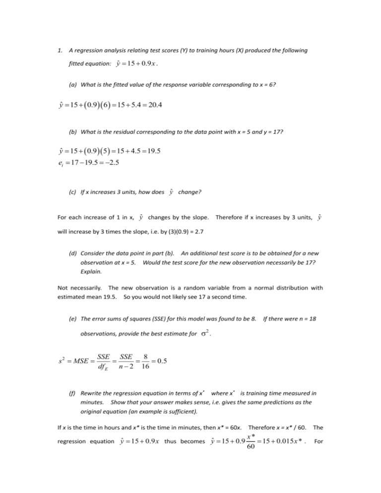
1. A regression analysis relating test scores (Y) to training hours (X) produced the following
fitted equation: yˆ  15  0.9 x .
(a) What is the fitted value of the response variable corresponding to x = 6?
yˆ  15   0.9 6  15  5.4  20.4
(b) What is the residual corresponding to the data point with x = 5 and y = 17?
yˆ  15   0.9  5  15  4.5  19.5
ei  17  19.5  2.5
(c) If x increases 3 units, how does ŷ change?
For each increase of 1 in x, ŷ changes by the slope. Therefore if x increases by 3 units, ŷ
will increase by 3 times the slope, i.e. by (3)(0.9) = 2.7
(d) Consider the data point in part (b). An additional test score is to be obtained for a new
observation at x = 5. Would the test score for the new observation necessarily be 17?
Explain.
Not necessarily. The new observation is a random variable from a normal distribution with
estimated mean 19.5. So you would not likely see 17 a second time.
(e) The error sums of squares (SSE) for this model was found to be 8. If there were n = 18
observations, provide the best estimate for  .
2
s 2  MSE 
SSE SSE
8


 0.5
df E n  2 16
(f) Rewrite the regression equation in terms of x* where x* is training time measured in
minutes. Show that your answer makes sense, i.e. gives the same predictions as the
original equation (an example is sufficient).
If x is the time in hours and x* is the time in minutes, then x* = 60x. Therefore x = x* / 60. The
regression equation yˆ  15  0.9 x thus becomes yˆ  15  0.9
x*
 15  0.015 x * .
60
For
example, if x = 2 hours then x* = 120 minutes.
The original equation would give
yˆ  15  0.9  2  15  1.8  16.8
new
,
and
the
equation
would
give
yˆ  15  0.015 120  15  1.8  16.8. . Thus the two equations give the same answer.
2. Explain the difference between the following two equations:
Ŷ  b0  b1 X
Y  0  1 X  
The first equation is the fitted regression line which describes the linear relationship between the
mean of the response variable (fitted value) and the explanatory variable X. The second
equation is the linear model which describes the relationship between the observed (X,Y) pairs.
Not all the pairs will fall directly on a line as they will in the first equation, as indicated by the
error term. In the first equation, the values b0 and b1 are known values obtained from the data,
while in the second equation, the parameters 1 and 0 are unknown.
3. Consider Figure 1.3 in KNNL. If only the data over years 8 – 15 were considered, a
reasonable linear fit could be obtained. This model, however, would profoundly over-predict
the steroid level when x = 25 years. Use this result in explaining what is meant by “scope of
model”.
“Scope of model” refers to limiting inference to only the region of X where you have data (and
where the model appears to hold). There is no guarantee that the relationship is linear over the
entire range of X where you do not have any data.