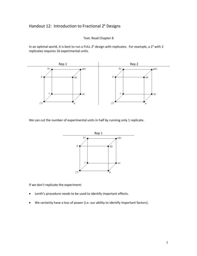
Handout 12: Introduction to Fractional 2k Designs
Text: Read Chapter 8
In an optimal world, it is best to run a FULL 2k design with replicates. For example, a 23 with 2
replicates requires 16 experimental units.
Rep 1
Rep 2
We can cut the number of experimental units in half by running only 1 replicate.
Rep 1
If we don’t replicate the experiment:

Lenth’s procedure needs to be used to identify important effects.

We certainly have a loss of power (i.e. our ability to identify important factors).
1
Fractional Factorials
As the number of factors in a 2k factorial design increases, the number of runs required for a
complete replicate is often more than the experimenter can handle. Can we cut the number of
experimental units even more? In short, the answer is yes—we will use a FRACTION of the full
factorial design. However, we do lose some information in the process.
Consider one slice of the design cube for a 23 design…
Slicing the cube according to
Factor A
Running only
Factor A = Low
Running only
Factor A = High
Running only one of these settings does not allow us to
measure the effect of Factor A
Try another slice of the cube…
Slicing the cube according to
Factor B
Running only
Factor B = Low
Running only
Factor B = High
Running only one of these settings does not allow us to
measure the effect of Factor B
2
A better method of slicing the cube…
Slicing the cube according to Factor ABC=High
Slicing the cube according to Factor ABC=Low
How do we determine which information is lost?
The +1/-1 matrix for the 8 treatment combinations is shown below.
Next, sort this matrix with respect to the ABC column.
3
If we run only Factor ABC=High, then we only use the top 4 rows of our +1/-1 matrix.
Note that the full factorial requires 23 runs; however, this design requires 23-1 = 4 runs. In
general, a one-half fraction of the 23 design is called a 23-1 design.
Since the identity column I always contains +1, we call I=ABC the defining relation for this
design.
Running an experiment in this fashion means we will not be able to distinguish between certain
effects. Columns that have the same plus/minus combinations are said to be aliased.
Factor
is aliased with
I
A
B
C
Likewise, if we use the bottom half of the +1/-1 matrix, we find the following.
Determine the alias structure when Factor ABC = Low is used
Factor
is aliased with
4
I
-ABC
A
B
C
What does it mean if effects are aliased? Consider the first design (with ABC = High). Here, it is
impossible to differentiate between A and BC, B and AC, and C and AB. In fact, when we
estimate A, B, and C, we are really estimating A+BC, B+AC, and C+AB.
The alias structure for this design can also be determined using the defining relation
I = ABC. To find aliases for any effect, multiply that effect by this defining relation:
Now, consider the second design (with ABC = Low). Here, the defining relation is given by I = ABC; thus, the aliases are found as follows:
So, when we estimate A, B, and C with this fractional design, we are really estimating
A - BC, B - AC, and C - AB.
The Concept Of Design Resolution
A design is of resolution R if no p-factor effect is aliased with another effect containing less than
R-p factors.

Resolution III Designs
5
These consist of designs in which no main effects (i.e. A, B, C, etc) are aliased
with any other main effects. It is possible that main effects are aliased with
two-factor interactions and two-factor interactions may be aliased with other
two-factor interactions.

Resolution IV Designs
These consist of designs in which no main effects are aliased with any other
main effects or with any two-factor interaction. It is possible that two-factor
interactions are aliased with other two-factor interactions.

Resolution V Designs
These consist of designs in which no main effects or two-factor interactions are
aliased with any other main effect or any other two-factor interaction. It is
possible that two-factor interactions are aliased with other three-factor
interactions.
Questions:
1. What is the design resolution of the previous example?
2. Do we want the resolution of a design to be high or low? Explain.
6
Minitab and Aliasing…
Let’s begin by working through the previous example in Minitab.
Using Default Generators…
The output on the spreadsheet…
7
The output in Minitab’s Session Window…
Notice, Minitab gives us the complete alias structure in the session window.
Comment:
In this example, we considered running only Factor ABC = High, and we determined that
the intercept was aliased with ABC.
I  ABC
As discussed earlier, an easy way to determine which effect is aliased with C is to
multiple both sides of the defining relations by C, which yields
C * I  C * ABC
C  ABC 2
C  AB
when mod 2 arithmetic is used.
Questions:
1. Verify the aliasing of factor A as shown in Minitab.
2. Verify the aliasing of factor B as shown in Minitab.
Using the information under the Display Available Designs tab in Minitab…
8
Comment:
Suppose three factors are under investigation and the budget allows for 8
experimental units. The question becomes “Is it better to run two replicates of a
one-half fraction of a 23 design (i.e. 23-1 design) or one replicate of 23 full design?”.
9
Constructing a 25 Fractional Design
Suppose we are conducting an experiment with five factors, and there are only 16 experimental
units available. Therefore, we have the choice to use either a Resolution III or Resolution V
design.
First, look the Resolution V Design…
10
Alias Information from Minitab’s Session window…
Questions:
1. Verify at least two of the aliasing arrangements from using the defining relation:
I  ABCDE
2. Verify that this design is indeed a Resolution V design.
Next, looking at the Resolution III Design…
11
Alias Information from Minitab’s Session window…
Questions:
1. How do you know this is a Resolution III design?
2. Would we consider this design to be “better” or “worse” than the previous design?
Why?
12
Another Example
Consider the following example. There are four factors under consideration.
This design in Minitab with the data….
Minitab’s Session window shows the alias structure
Fractional Factorial Design
Factors: 4 Base Design:
4, 8 Resolution: IV
Runs: 8 Replicates:
1 Fraction: 1/2
Blocks: 1 Center pts (total): 0
Design Generators: D = ABC
Alias Structure
I + ABCD
A + BCD
B + ACD
C + ABD
D + ABC
AB + CD
AC + BD
AD + BC
Lenth’s procedure fails to identify any important effects (which should be expected
because we have very few runs in this experiment).
13
Consider the fitted model effects from Minitab:
Factorial Fit: filtration rate versus A, B, C, D
Estimated Effects and Coefficients for filtration rate (coded units)
Term
Effect Coef
Constant
70.750
A
19.000 9.500
B
1.500 0.750
C
14.000 7.000
D
16.500 8.250
A*B
-1.000 -0.500
A*C
-18.500 -9.250
A*D
19.000 9.500
Questions:
1. How do the estimates of main effects compare to each other?
2. What do you conclude about Factor B relative to the other factors?
Comment: If Factor B is not important and is not included in the model, we are actually
collapsing our cubes over Factor B.
14
Removing Effect B from the model…
15
The overall ANOVA table
Factorial Fit: Filtration Rate versus A, C, D
Estimated Effects and Coefficients for Filration Rate (coded units)
Term
Effect Coef SE Coef
T P
Constant
70.750 0.6374 111.00 0.000
A
19.000 9.500 0.6374 14.90 0.004
C
14.000 7.000 0.6374 10.98 0.008
D
16.500 8.250 0.6374 12.94 0.006
A*C
-18.500 -9.250 0.6374 -14.51 0.005
A*D
19.000 9.500 0.6374 14.90 0.004
S = 1.80278 R-Sq = 99.79% R-Sq(adj) = 99.26%
Analysis of Variance for Filration Rate (coded units)
Source
DF Seq SS Adj SS Adj MS
F P
Main Effects
3 1658.50 1658.50 552.833 170.10 0.006
2-Way Interactions 2 1406.50 1406.50 703.250 216.38 0.005
Residual Error
2 6.50 6.50 3.250
Total
7 3071.50
These effects are important (especially considering the above is based only on 2 df for error).
Normal Probability Plot of the Standardized Effects
(response is filtration rate, Alpha = .05)
99
Effect Ty pe
Not Significant
Significant
95
90
AD
Percent
80
70
A
60
50
40
30
F actor
A
C
D
N ame
A
C
D
D
C
20
AC
10
5
1
-15
-10
-5
0
5
Standardized Effect
10
15
16
Residuals Plots…
Residual Plots for filtration rate
Normal Probability Plot of the Residuals
Residuals Versus the Fitted Values
99
1.0
Residual
Percent
90
50
10
1
-2
-1
0
Residual
1
2
40
Histogram of the Residuals
60
80
Fitted Value
100
Residuals Versus the Order of the Data
1.0
1.5
Residual
Frequency
0.0
-0.5
-1.0
2.0
1.0
0.5
0.0
0.5
0.5
0.0
-0.5
-1.0
-1.5
-1.0
-0.5
0.0
0.5
Residual
1.0
1.5
1
2
3
4
5
6
Observation Order
7
8
17
Fitted Mean Interaction Plots…
Interaction Plot (data means) for filtration rate
-1
1
-1
1
100
75
A
-1
1
A
50
100
75
C
-1
1
C
50
D
18