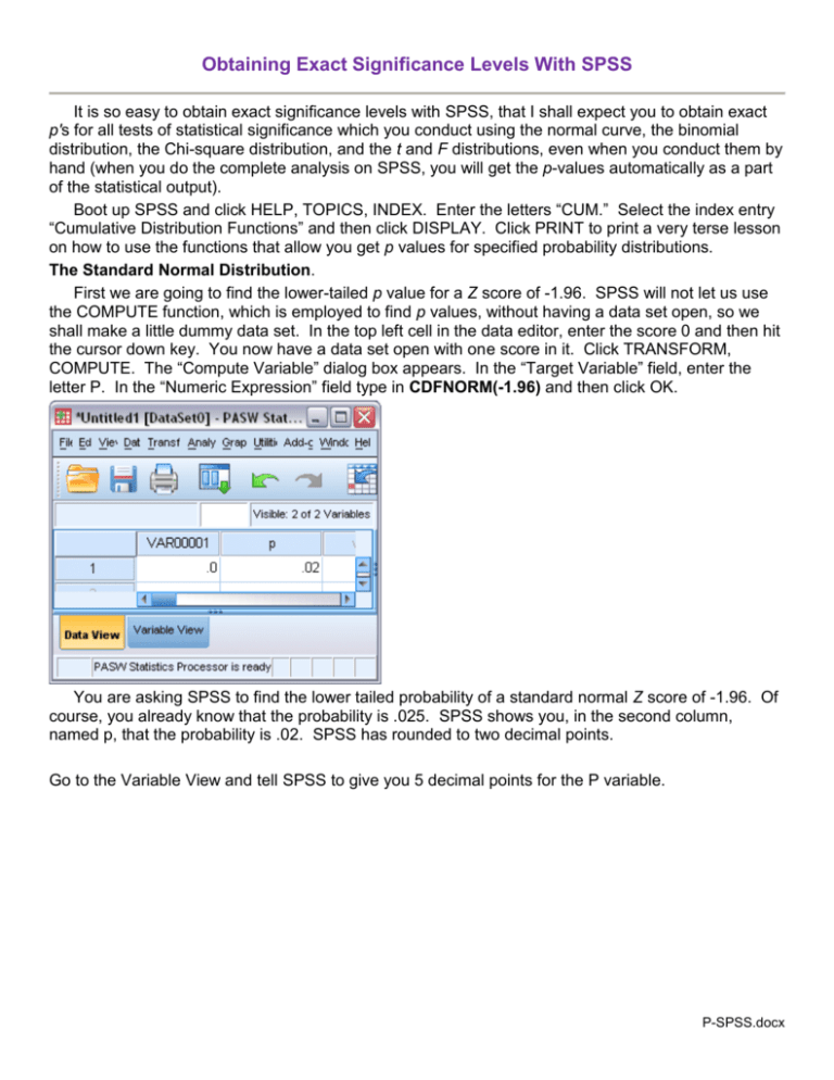
Obtaining Exact Significance Levels With SPSS
It is so easy to obtain exact significance levels with SPSS, that I shall expect you to obtain exact
p's for all tests of statistical significance which you conduct using the normal curve, the binomial
distribution, the Chi-square distribution, and the t and F distributions, even when you conduct them by
hand (when you do the complete analysis on SPSS, you will get the p-values automatically as a part
of the statistical output).
Boot up SPSS and click HELP, TOPICS, INDEX. Enter the letters “CUM.” Select the index entry
“Cumulative Distribution Functions” and then click DISPLAY. Click PRINT to print a very terse lesson
on how to use the functions that allow you get p values for specified probability distributions.
The Standard Normal Distribution.
First we are going to find the lower-tailed p value for a Z score of -1.96. SPSS will not let us use
the COMPUTE function, which is employed to find p values, without having a data set open, so we
shall make a little dummy data set. In the top left cell in the data editor, enter the score 0 and then hit
the cursor down key. You now have a data set open with one score in it. Click TRANSFORM,
COMPUTE. The “Compute Variable” dialog box appears. In the “Target Variable” field, enter the
letter P. In the “Numeric Expression” field type in CDFNORM(-1.96) and then click OK.
You are asking SPSS to find the lower tailed probability of a standard normal Z score of -1.96. Of
course, you already know that the probability is .025. SPSS shows you, in the second column,
named p, that the probability is .02. SPSS has rounded to two decimal points.
Go to the Variable View and tell SPSS to give you 5 decimal points for the P variable.
P-SPSS.docx
2
Return to the data view and you see that the p is .02500.
Binomial Distribution
You wish to determine if mothers can identify their babies from the scent of the baby. Your
research participants are mothers and their newborn babies in a maternity ward. You take shirts that
the babies have worn for a while and stuff them into cardboard tubes. To each of 17 mothers you
present two tubes, one that contains her baby’s shirt, one that contains another baby’s shirt. You ask
her to sniff both tubes and ‘guess’ which one has her baby’s shirt in it. Thirteen of the 17 mothers
correctly identify their baby, four do not. This example is based on actual research, by the way. If
mothers really cannot identify their babies by scent alone, but just guess on a task like this, what is
the probability of as few as 4 out of 17 having guessed incorrectly? This is a question that involves
the binomial distribution, a distribution in which the variable has only two possible outcomes (in this
case, a correct identification or an incorrect identification). To obtain the binomial probability, we
TRANSFORM, COMPUTE, and tell SPSS to set the value of P to CDF.BINOM(4,17,.5). The 4 is the
observed number of failures correctly to identify the baby, the 17 is the number of mothers who tried
to do it, and the .5 is the probability of correctly identifying the baby if the mother was just “blindly
guessing.” SPSS tells us that the probability of getting that few correct identifications if the mothers
were really just blindly guessing is only .025. That should convince us that mothers really can identify
their babies on the basis of scent alone.
3
Chi-Square Distribution
Suppose that we wish to determine whether or not three different types of therapy differ with
respect to their effectiveness in relieving symptoms of chronic anxiety. Our independent variable is
type of therapy and the dependent variable is whether or not the patient reports having experienced a
reduction in anxiety after three months of treatment. We analyze the contingency table with a
Pearson Chi-Square and obtain a value of 5.99 for the test statistic. Is this significant? In the
“Numeric Expression” field of the Compute Variable dialog box we enter CDF.CHISQ(5.99,2) and
click OK. SPSS tells us that the lower-tailed p is .94996 -- but we need an upper-tailed p for this
application of 2, so we subtract from one and obtain a p of .05004. Technically, this is not quite less
than or equal to the holy criterion of .05, but we round it off to four decimal points and conclude that
the three types of therapy do differ significantly in effectiveness.
Student’s t Distribution
We wish to determine whether sick animals who have been given a certain medical treatment
differ from those who have received a placebo treatment with respect to the severity of their illness
after treatment. A t test yields a value of t = 2.23 on 10 degrees of freedom. To get the p value, we
enter in the “Numeric Expression" field of the Compute Variable dialog box CDF.T(-2.23,10) and
obtain a one-tailed p of .02492. Since we desire a two-tailed p, we double this, obtaining .0498, and
conclude that the treated animals did differ significantly from those who received only a placebo.
F Distribution
We have conducted an Analysis of Variance to determine if students in three different majors
differ with respect to how many hours they say they spend studying in a typical week. We obtain a F
of 3.33 on 2, 27 degrees of freedom. To get the p value, we enter in the “Numeric Expression" field of
the Compute Variable dialog box CDF.F(3.33,2,27) and obtain a lower-tailed p value of .95203.
Since this application of the F statistic requires an upper-tailed p, we subtract from one and obtain a p
value of .048. We conclude that the majors do differ significantly on how many hours they report they
spend studying.
If you have more than one value of F, you can get all of the p values in one run by entering F, df1,
and df2 as data and then pointing the CDF function to those variables, as shown below. Notice that I
had SPSS subtract from 1 for me.
4
Return to Wuensch’s SPSS Lessons Page
Karl L. Wuensch, Dept. of Psychology,
East Carolina University, Greenville, NC 27858 USA
July, 2014