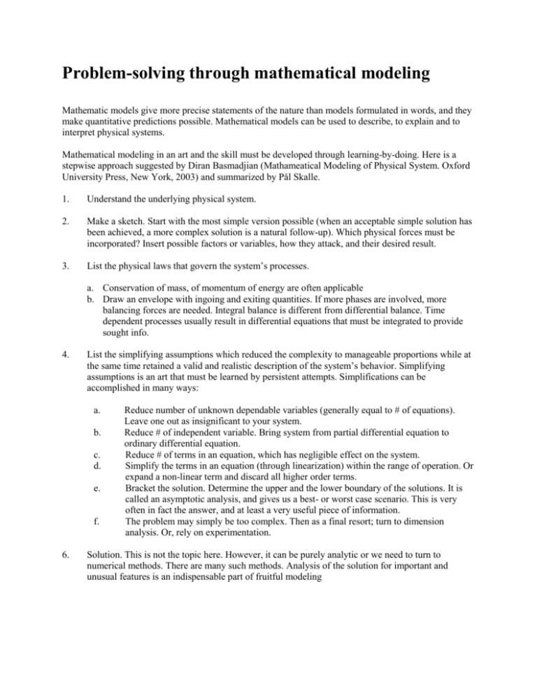
Problem-solving through mathematical modeling
Mathematic models give more precise statements of the nature than models formulated in words, and they
make quantitative predictions possible. Mathematical models can be used to describe, to explain and to
interpret physical systems.
Mathematical modeling in an art and the skill must be developed through learning-by-doing. Here is a
stepwise approach suggested by Diran Basmadjian (Mathameatical Modeling of Physical System. Oxford
University Press, New York, 2003) and summarized by Pål Skalle.
1.
Understand the underlying physical system.
2.
Make a sketch. Start with the most simple version possible (when an acceptable simple solution has
been achieved, a more complex solution is a natural follow-up). Which physical forces must be
incorporated? Insert possible factors or variables, how they attack, and their desired result.
3.
List the physical laws that govern the system’s processes.
a. Conservation of mass, of momentum of energy are often applicable
b. Draw an envelope with ingoing and exiting quantities. If more phases are involved, more
balancing forces are needed. Integral balance is different from differential balance. Time
dependent processes usually result in differential equations that must be integrated to provide
sought info.
4.
List the simplifying assumptions which reduced the complexity to manageable proportions while at
the same time retained a valid and realistic description of the system’s behavior. Simplifying
assumptions is an art that must be learned by persistent attempts. Simplifications can be
accomplished in many ways:
a.
b.
c.
d.
e.
f.
6.
Reduce number of unknown dependable variables (generally equal to # of equations).
Leave one out as insignificant to your system.
Reduce # of independent variable. Bring system from partial differential equation to
ordinary differential equation.
Reduce # of terms in an equation, which has negligible effect on the system.
Simplify the terms in an equation (through linearization) within the range of operation. Or
expand a non-linear term and discard all higher order terms.
Bracket the solution. Determine the upper and the lower boundary of the solutions. It is
called an asymptotic analysis, and gives us a best- or worst case scenario. This is very
often in fact the answer, and at least a very useful piece of information.
The problem may simply be too complex. Then as a final resort; turn to dimension
analysis. Or, rely on experimentation.
Solution. This is not the topic here. However, it can be purely analytic or we need to turn to
numerical methods. There are many such methods. Analysis of the solution for important and
unusual features is an indispensable part of fruitful modeling