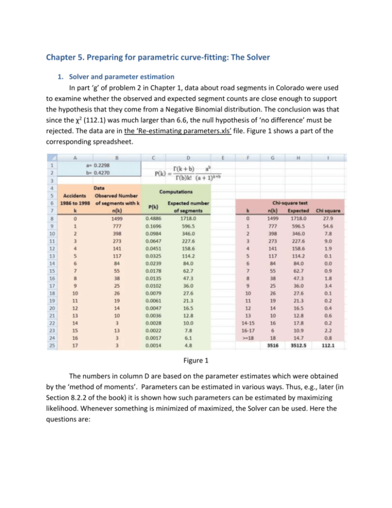
Chapter 5. Preparing for parametric curve-fitting: The Solver
1. Solver and parameter estimation
In part ‘g’ of problem 2 in Chapter 1, data about road segments in Colorado were used
to examine whether the observed and expected segment counts are close enough to support
the hypothesis that they come from a Negative Binomial distribution. The conclusion was that
since the χ2 (112.1) was much larger than 6.6, the null hypothesis of ‘no difference’ must be
rejected. The data are in the ‘Re-estimating parameters.xls’ file. Figure 1 shows a part of the
corresponding spreadsheet.
Figure 1
The numbers in column D are based on the parameter estimates which were obtained
by the ‘method of moments’. Parameters can be estimated in various ways. Thus, e.g., later (in
Section 8.2.2 of the book) it is shown how such parameters can be estimated by maximizing
likelihood. Whenever something is minimized of maximized, the Solver can be used. Here the
questions are:
a. What would be the parameters ‘a’ and ‘b’ if estimated by minimizing χ2? Doing
so makes some sense since the χ2 =
(observed−expected)2
expected
is commonly used to
describe goodness-of-fit.
b. How good is the resulting fit and whether the ‘no difference’ null hypothesis
would still be rejected?
2. SOLVER and the ‘Calibration Factor’
To make use of the Safety Performance Functions in the Highway Safety Manual one has
to have a jurisdiction-specific ‘calibration factor’, C defined as:
C=
∑all sites observed crashes
∑all sites crashes predicted by the HSM without the calibration factor
The purpose of the calibration factor is to account for whatever differences there are
between the jurisdiction where the SPFs are to be used and the jurisdiction (and time) from
which the data for the SPF came.
To estimate the ‘C’ a set of representative sites has to be chosen at which additional
information has to be collected. This information is about some traits specified in the HSM
which are needed to compute the predicted crashes in the denominator of the above equation.
The summation is over all sites for which this information is available.
In one such calibration exercise a State collected data at 350 segments of multilane rural roads,
used the data to compute the predicted-by-the-HSM yearly crash frequency, and ascertained
the number of observed crashes in three years. The data are in the ‘Predicted and Observed.xls’
file. The question is whether C is the same for all sites, irrespective of what their traits are. To
answer:
(a) Determine the overall C.
(b) Prepare a graph with ‘Predicted/year’ on the horizontal axis and ‘Observed in three
years’ on the vertical axis. If the points form a straight line this is an indication the ‘C’ is
constant. Does the relationship look like a straight line?
(c) To check whether it is a straight line estimate the parameters β0 and β1 of the model
equation
Expected Crashes at site i, μi = β0 (Predicted by HSM crashes at site i)β1
If it is a straight line then β0/3 should be close to C and β1 should be close to 11.
1
Because the observed crashes are for three years β 0 is divided by 3.
It is here where Solver comes in. For each site we have the count of accidents, k, and
also the predicted-by –HSM value. As will be shown in Chapter 8, the natural logarithm of the
(abridged) likelihood of observing the accident counts k1, k2, …,k350 is:
350
∑(−μi ) + k i ln(μi )
i=1
Replacing the μ’s by the model equation β0 (Predicted by HSM accidentsi )β1 turns the
expression into a function of β0 and β1. Fitting this model equation amounts to finding those
values of β0 and β1 which maximize the likelihood of observing these accident counts.
Is the function a straight line? What are the implications of your finding for the HSM
calibration procedure?