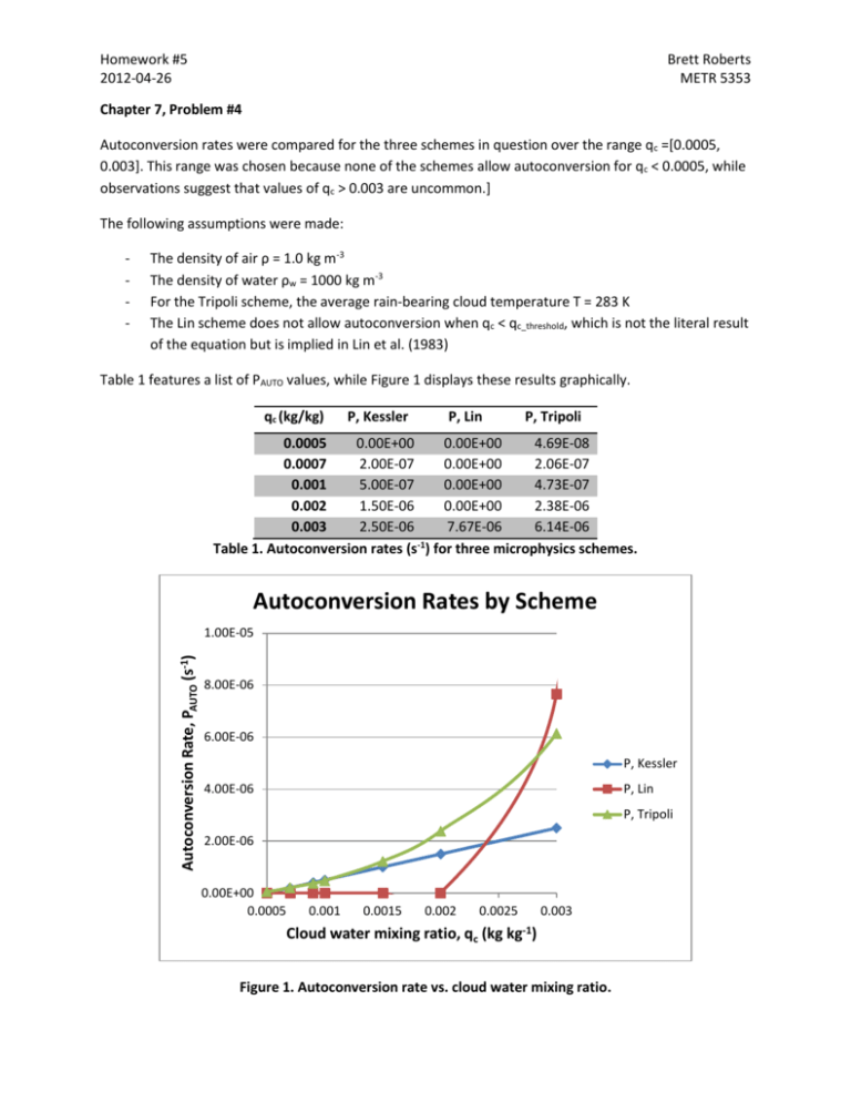
Homework #5
2012-04-26
Brett Roberts
METR 5353
Chapter 7, Problem #4
Autoconversion rates were compared for the three schemes in question over the range qc =[0.0005,
0.003]. This range was chosen because none of the schemes allow autoconversion for qc < 0.0005, while
observations suggest that values of qc > 0.003 are uncommon.]
The following assumptions were made:
-
The density of air ρ = 1.0 kg m-3
The density of water ρw = 1000 kg m-3
For the Tripoli scheme, the average rain-bearing cloud temperature T = 283 K
The Lin scheme does not allow autoconversion when qc < qc_threshold, which is not the literal result
of the equation but is implied in Lin et al. (1983)
Table 1 features a list of PAUTO values, while Figure 1 displays these results graphically.
qc (kg/kg)
P, Kessler
P, Lin
P, Tripoli
0.0005
0.00E+00
0.00E+00
4.69E-08
0.0007
2.00E-07
0.00E+00
2.06E-07
0.001
5.00E-07
0.00E+00
4.73E-07
0.002
1.50E-06
0.00E+00
2.38E-06
0.003
2.50E-06
7.67E-06
6.14E-06
-1
Table 1. Autoconversion rates (s ) for three microphysics schemes.
Autoconversion Rates by Scheme
Autoconversion Rate, PAUTO (s-1)
1.00E-05
8.00E-06
6.00E-06
P, Kessler
4.00E-06
P, Lin
P, Tripoli
2.00E-06
0.00E+00
0.0005
0.001
0.0015
0.002
0.0025
Cloud water mixing ratio, qc (kg
0.003
kg-1)
Figure 1. Autoconversion rate vs. cloud water mixing ratio.
Homework #5
2012-04-26
Brett Roberts
METR 5353
The Kessler and Tripoli calculations for autoconversion rate are relatively similar for low values of qc (qc <
0.002); for higher values, the Tripoli calculation becomes increasingly larger than Kessler. The Lin
calculation behaves much differently, not activating at all until qc > 0.002. Above its threshold, however,
it ramps up much more rapidly than the other two schemes. At qc = 0.003, the Tripoli scheme calculates
PAUTO more than 100% larger than Kessler, while the Lin value is over 200% larger.
Note that all calculations were performed using formulas in Microsoft Excel, owing to the number of
calculations needed. (This applies to the remaining problems, as well).
Chapter 7, Problem #6
Accretion rates were compared for the three schemes in question over the range qr = [0, 0.01].
Numerous assumptions were made in this assessment:
-
For the Kessler scheme, the collection efficiency E = 1 in all cases
For all schemes, the cloud water mixing ratio qc = 0.002 was chosen arbitrarily, since none was
specified
The density of air ρ = 1.0 kg m-3
The density of water ρw = 1000 kg m-3
The rain intercept parameter n0r = 8x106 m-4, per Marshall and Palmer (1948).
Table 2 features a list of PACCR values, while Figure 2 displays these values graphically.
With all else constant, these three schemes increase accretion linearly with rain water mixing ratio; the
only difference in their behaviors is the rate of increase (slope). The Schultz scheme has the highest
slope, followed by Tripoli, with Kessler the slowest-increasing. Therefore, the larger qr becomes, the
more difference is found between the three schemes.
qr (kg/kg)
P, Kessler
P, Tripoli
P, Schultz
0.0001
1.04E-06
1.07E-06
3.40E-06
0.0003
2.95E-06
3.20E-06
1.02E-05
0.0005
4.78E-06
5.33E-06
1.70E-05
0.0007
6.59E-06
7.46E-06
2.38E-05
0.001
9.24E-06
1.07E-05
3.40E-05
0.0015
1.36E-05
1.60E-05
5.10E-05
0.002
1.79E-05
2.13E-05
6.80E-05
0.003
2.62E-05
3.20E-05
1.02E-04
0.005
4.26E-05
5.33E-05
1.70E-04
0.01
8.24E-05
1.07E-04
3.40E-04
-1
Table 2. Accretion rates (s ) for three microphysics schemes.
Homework #5
2012-04-26
Brett Roberts
METR 5353
Accretion Rates by Scheme
4.00E-04
Accretion Rate, PACCR (s-1)
3.50E-04
3.00E-04
2.50E-04
2.00E-04
P, Kessler
P, Tripoli
1.50E-04
P, Schultz
1.00E-04
5.00E-05
0.00E+00
0
0.002
0.004
0.006
0.008
0.01
Rain water mixing ratio, qr (kg kg-1)
Figure 2. Accretion rate vs. rain water mixing ratio.
Chapter 9, Problem #2
Downwelling longwave radiation was calculated using the method proposed by Harshvardham and
Weinman (1982). The cloud fraction b was varied from 0.2 to 1, while the cloud aspect ratio a was varied
from 1 to 5. The results are tabulated in Table 3.
b
0.2
0.4
0.6
0.8
1
330.17
334.6491
337.4776
339.426
340.8497
338.6364
342.2107
344.0745
345.2186
345.9924
343.9341
346.1283
347.1568
347.7535
348.1432
347.4928
348.4729
348.9021
349.143
349.2972
350
350
350
350
350
a
1
2
3
4
5
Table 3. Downwelling radiation (W m-2) for varying cloud conditions.
The results indicate that cloud aspect ratio is most critical when cloud cover is relatively low (but
nonzero, of course). The deviation from cloudy-sky conditions (FD = 350 W m-2) at b = 0.2 over the range
a = [1,5] varies by about 100% (~341 W m-2 vs. ~330 W m-2).
Homework #5
2012-04-26
Brett Roberts
METR 5353
Chapter 9, Problem #3
Linear interpolation of the results in Table 3 suggests that an error in b of 30%, with a range of b =
[0.2,0.5], may result in an error of ~10 W m-2 in FD. If the 30% error is centered around a higher cloudcover value, covering the range b = [0.7,1], then the resultant radiation error is reduced to ~2 W m-2.
This is, of course, dependent upon the FD-clear and FD-cloudy values assumed for this problem.
The worst-case error of 10 W m-2 is certainly a noteworthy error in the radiation budget, though it is not
likely to be catastrophic for the model, given that it’s one to two orders of magnitude smaller than the
radiation terms themselves (e.g., FD ~ 350 W m-2). On the first exam, it was found that a constant 50 W
m-2 error in the radiation budget resulted in a mixed-layer temperature error of ~2 K by the end of a day.
Given that our 30% cloud-cover error is unlikely to persist throughout an entire diurnal cycle, and that
its error in the radiation budget is only ~10 W m-2, the effect upon boundary-layer temperature is
unlikely to be particularly noteworthy.