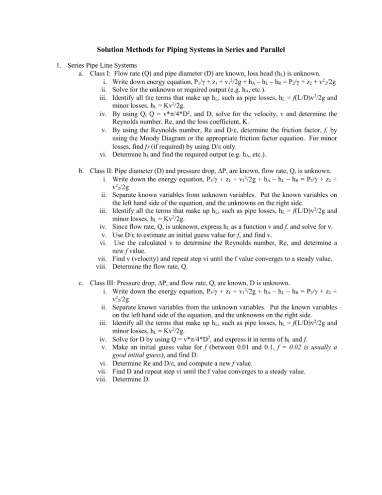
Solution Methods for Piping Systems in Series and Parallel
1. Series Pipe Line Systems
a. Class I: Flow rate (Q) and pipe diameter (D) are known, loss head (hL) is unknown.
i. Write down energy equation, P1/ + z1 + v12/2g + hA – hL – hR = P2/ + z2 + v22/2g
ii. Solve for the unknown or required output (e.g. hA, etc.).
iii. Identify all the terms that make up h L, such as pipe losses, hL = f(L/D)v2/2g and
minor losses, hL = Kv2/2g.
iv. By using Q, Q = v*/4*D2, and D, solve for the velocity, v and determine the
Reynolds number, Re, and the loss coefficient, K.
v. By using the Reynolds number, Re and D/, determine the friction factor, f, by
using the Moody Diagram or the appropriate friction factor equation. For minor
losses, find fT (if required) by using D/ only.
vi. Determine hL and find the required output (e.g. hA, etc.).
b. Class II: Pipe diameter (D) and pressure drop, P, are known, flow rate, Q, is unknown.
i. Write down the energy equation, P1/ + z1 + v12/2g + hA – hL – hR = P2/ + z2 +
v22/2g
ii. Separate known variables from unknown variables. Put the known variables on
the left hand side of the equation, and the unknowns on the right side.
iii. Identify all the terms that make up h L, such as pipe losses, hL = f(L/D)v2/2g and
minor losses, hL = Kv2/2g.
iv. Since flow rate, Q, is unknown, express hL as a function v and f, and solve for v.
v. Use D/to estimate an initial guess value for f, and find v.
vi. Use the calculated v to determine the Reynolds number, Re, and determine a
new f value.
vii. Find v (velocity) and repeat step vi until the f value converges to a steady value.
viii. Determine the flow rate, Q.
c. Class III: Pressure drop, P, and flow rate, Q, are known, D is unknown.
i. Write down the energy equation, P1/ + z1 + v12/2g + hA – hL – hR = P2/ + z2 +
v22/2g
ii. Separate known variables from the unknown variables. Put the known variables
on the left hand side of the equation, and the unknowns on the right side.
iii. Identify all the terms that make up h L, such as pipe losses, hL = f(L/D)v2/2g and
minor losses, hL = Kv2/2g.
iv. Solve for D by using Q = v*/4*D2, and express it in terms of hL and f.
v. Make an initial guess value for f (between 0.01 and 0.1, f = 0.02 is usually a
good initial guess), and find D.
vi. Determine Re and D/, and compute a new f value.
vii. Find D and repeat step vi until the f value converges to a steady value.
viii. Determine D.
2. Parallel Pipe Line Systems
a. Two branches, total flow rate, Q, and D are known. Total pressure drop (or total head)
and individual branch flow rates are unknown.
i. Identify all the terms that make up h L, such as pipe losses, hL = f(L/D)v2/2g and
minor losses, hL = Kv2/2g for each branch.
ii. Since the flow rate for each branch, Qi, is unknown, express hL for each branch as
a function of velocity, v1 or v2 and f1 or f2.
iii. Equate the two hL’s and express them in terms of f1 and f2 and v1 or v2. Solve for
one velocity.
iv. Make an initial guess value for f1 and f2 (between 0.01 and 0.1), and by using
Qtotal = Q1 + Q2, find v1 and v2, determine Re1 and Re2, D1/1 and D2/2, and find
f1 and f2.
v. Repeat steps iii and iv until f1 and f2 converge to steady values.
vi. Determine Q1 and Q2, and h1 and h2.
Note: If k values are given for each branch (hL1 = K1v12/2g and hL2 = K2v22/2g), then solve for
one of the velocities by equating hL1 = hL2 and using Qtotal = Q1 + Q2. Then determine Q1 and Q2.
b. Two branches, total pressure drop (or total head) is known. Total flow rate and
individual branch flow rates are unknown.
i. Identify all the terms that make up h L, such as pipe losses, hL = f(L/D)v2/2g and
minor losses, hL = Kv2/2g for each branch.
ii. Since the flow rate for each branch, Qi, is unknown, express v1 and v2 for each
branch as a function of h1 and h2, respectively.
iii. Since the pressure drop is known, find h1 and h2.( hL = h1 = h2)
iv. Determine v1 and v2 by making initial guesses for f1 and f2 (between 0.01 and
0.1), and by using Qtotal = Q1 + Q2, if necessary. Once v1 and v2 are computed,
determine Re1 and Re2, D1/1 and D2/2, and find f1 and f2.
v. Repeat steps iv until f1 and f2 converge to steady values.
vi. Determine Q1, Q2 and QTotal, and h1 and h2.
Note: If k values are given for each branch (hL1 = K1v12/2g and hL2 = K2v22/2g), then find each
velocity v1 and v2 and find Qtotal = Q1 + Q2.