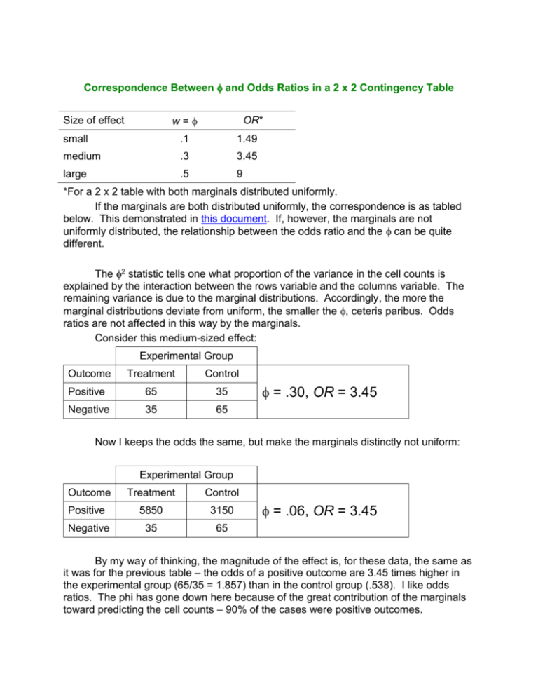
Correspondence Between  and Odds Ratios in a 2 x 2 Contingency Table
w=
Size of effect
OR*
small
.1
1.49
medium
.3
3.45
large
.5
9
*For a 2 x 2 table with both marginals distributed uniformly.
If the marginals are both distributed uniformly, the correspondence is as tabled
below. This demonstrated in this document. If, however, the marginals are not
uniformly distributed, the relationship between the odds ratio and the  can be quite
different.
The 2 statistic tells one what proportion of the variance in the cell counts is
explained by the interaction between the rows variable and the columns variable. The
remaining variance is due to the marginal distributions. Accordingly, the more the
marginal distributions deviate from uniform, the smaller the , ceteris paribus. Odds
ratios are not affected in this way by the marginals.
Consider this medium-sized effect:
Experimental Group
Outcome
Treatment
Control
Positive
65
35
Negative
35
65
 = .30, OR = 3.45
Now I keeps the odds the same, but make the marginals distinctly not uniform:
Experimental Group
Outcome
Treatment
Control
Positive
5850
3150
Negative
35
65
 = .06, OR = 3.45
By my way of thinking, the magnitude of the effect is, for these data, the same as
it was for the previous table – the odds of a positive outcome are 3.45 times higher in
the experimental group (65/35 = 1.857) than in the control group (.538). I like odds
ratios. The phi has gone down here because of the great contribution of the marginals
toward predicting the cell counts – 90% of the cases were positive outcomes.
So, which should you report,  or OR? I recommend reporting both and, when
the marginals are distinctly not uniform, explaining how  is greatly affected by
nonuniformity of the marginals but OR is not.
Here are some more examples. With uniform marginals, a phi of .1 corresponds
to an OR of 1.49. Here I increase the base rate of positive outcomes and the ratio of
the odds, keeping  at .1.
Experimental Group
Outcome
Treatment
Control
Positive
800
100
Negative
78
22
 = .10, OR = 2.26
With uniform marginals, a phi of .3 corresponds to an OR of 3.45. Here I
increase the base rate of positive outcomes and the ratio of the odds, keeping  at .3.
Experimental Group
Outcome
Treatment
Control
Positive
795
96
Negative
55
46
 = .30, OR = 6.93
With uniform marginals, a phi of .5 corresponds to an OR of 9. Here I increase
the base rate of positive outcomes and the ratio of the odds, keeping  at .5.
Experimental Group
Outcome
Treatment
Control
Positive
800
99
Negative
26
74
 = .50, OR = 23.00
In a very similar fashion, when comparing two groups’ means, the
correspondence between the standardized difference between means (Cohen’s d) and
the point-biserial correlation coefficient (when squared, a proportion of variance, also
known as eta-squared) depends on how much the within-group sample sizes differ from
each other. See my document Effect of n1/n2 on Estimated d and rpb.
Karl L. Wuensch, East Carolina University, November, 2009.