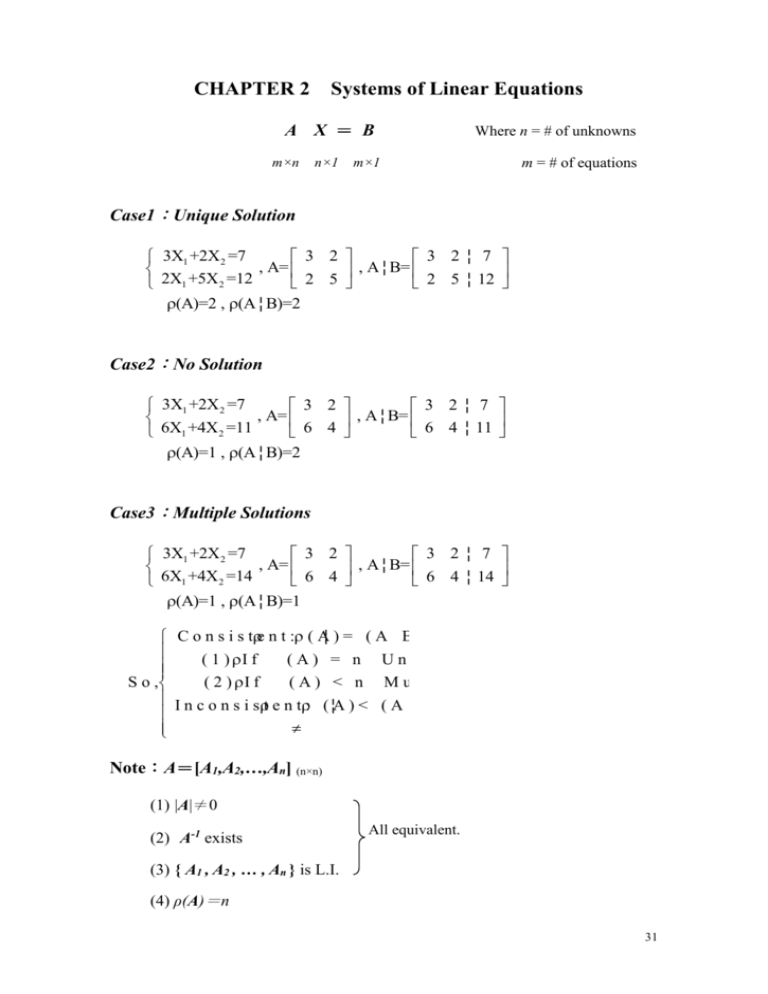
CHAPTER 2
Systems of Linear Equations
A X ＝ B
m×n
n×1
Where n = # of unknowns
m×1
m = # of equations
Case1：Unique Solution
 3X1 +2X 2 =7
 3 2 
 3 2 ¦ 7 
, A= 
, A ¦ B= 



 2 5 
 2 5 ¦ 12 
 2X1 +5X 2 =12
(A)=2 , (A ¦ B)=2
Case2：No Solution
 3X1 +2X 2 =7
 3 2 
 3 2 ¦ 7 
, A= 
,
A
¦
B=


 6 4 ¦ 11 
 6 4 


 6X1 +4X 2 =11
(A)=1 , (A ¦ B)=2
Case3：Multiple Solutions
 3X1 +2X 2 =7
 3 2 
 3 2 ¦ 7 
, A= 
, A ¦ B= 



 6 4 
 6 4 ¦ 14 
 6X1 +4X 2 =14
(A)=1 , (A ¦ B)=1
 C o n s i s te n t : ( A¦ ) = ( A B )

( 1 ) I f
(A) = n Unique Solu.

S o ,
( 2 ) I f
(A) < n Multiple Solu.
 I n c o n s i st e n t: ( ¦A ) < ( A B )



Note：A＝[A1,A2,…,An] (n×n)
(1) |A|≠0
(2) A-1 exists
All equivalent.
(3) { A1 , A2 , … , An } is L.I.
(4) ρ(A)＝n
31
Rule of Rank for AX＝B ( where m＝n )
ρ(A)＝ρ(A ¦ B)
1≦ρ(A)＜n
ρ(A)＝n
ρ(A)＜ρ(A ¦ B)
Multiple Solution：m－ρ(A) Partial Solution：m－ρ(A)
equations are redundant
equations must be removed to
and can be removed.
have a “partial solution”
Unique Solution：X＝A-1B
Impossible
 X1 +2X 2 -X3 =4

Ex：  2X1 +5X 2 +X3 =7  (A)=2 < n=3
 2X +4X -2X =8
1
2
3

max (A|B)-(A)
=3-2=1
 Solu. lie on 1-dim space
Intersect at a line.
 X1 +2X 2 -X3 =4

Ex：  4X1 +8X 2 -4X3 =16
 2X +4X -2X =8
1
2
3

max (A|B)-(A)
 (A)=1 < n=3
=3-1=2
 Solu. lie on 2-dim space
Intersect at a plane.
For consistent cases：
1. max ρ(A ¦ B)－ρ(A) describes the nature of solu.
 n-(A)  number of redundent equations
2. 
 m-(A)  ..................................................
For inconsistent cases：
ρ(A) indicates the # of equations that can be simultaneously satisfied by
any specific point.
32
Homogeneous Systems： AX＝0 ( B=0 )
 X1 -2X 2 +X3 =0

Ex：  3X1 +X 2 -2X3 =0
 2X +X +X =0
1
2
3

1. always consistent ( ρ(A)＝ρ( A | 0 ) )
2. If ρ(A)＝n , Unique Sole：X=A-1× 0 = 0
Otherwise, ρ(A)＜n , Multiple Solu. ( Nontrivial Solutions exist )
Unique Solu. ( X1 =X 2 =0 )
 X -X =0

(1)  1 2
(A)=2=n
 2X1  X 2  0
Multiple Solu. ( X1 =X 2 )
 X -X =0

(2)  1 2
(A)=1<2
 2X1  2X 2  0
Note：Suppose A is m×n
1. ρ(A)≦min(m, n)
2. If ρ(A)＝min(m, n) , then A is said to have full rank.
3. If A has full rank and m＞n , then A’A is m×n and ρ(A’A)＝n
 1 2 2 
Ex： A   2 1 4  , (A)=?


 3 1 6 
1 
2 
1  2   2  1   3
 3 
1 
 1 2 2 2 3

  21  2 4 3
 3   6 
1
2
3

2  0 
 4   0 
   
6  0 

0
0 ( - 2 a , 0 , 
a ) , a RA ) = 2

0
L.D.
33
(
Def：A matrix is in its reduced row echelon from ( rref ), if the following
conditions hold：
1. The zero rows if any , are the last rows of the matrix .
2. The first nonzero entry in a nonzero row is a one . It is called a leading one .
3. Each Column containing a leading one is a unit vector , ei , for some i .
4. The leading one in row p is to the left of the leading one in row q ,
whenever p< q .


Ex： 



1
0
0
0
0
1
0
0






 1 * * * 
Ex：  0 0 0 0 


 0 0 0 0 


Ex： 



1
0
0
0
*
0
0
0
0
0
0
0
0
0
1
0
0
1
0
0


Ex： 



1
0
0
0
*
0
0
0
0
1
0
0
0
0
1
0


Ex： 



1
0
0
0
*
0
0
0
0
0
0
0
0
0
*
0
*
*
*
0


 ( *：any number )















How to determine the rank of a matrix？
(1) Transform the matrix into its rref by expanded elementary row
operations (e.e.r.o.).
e.e.r.o.：
1. row i ×c ( c = constant )
2. add c ×( row i ) to row j
34
expanded elementary row operations (e.e.r.o)＝{elementary row operations(e.r.o.)}
∪{interchanging 2 rows}
(2) The rank of the matrix ＝ # of nonzero rows in its rref.
Ex：
(-1)
 0 1 1
 0 -1 -1

 0 1 1
 0 1 1
  0 0 0
 0 0 0
(-2)
1 1   0 1 1 1 1   0 1 1 0 0 
1 1    0 0 0 2 2    0 0 0 1 1 
1 2   0 0 0 0 1   0 0 0 0 1 
0 0 
1 0   (A)  3
0 1 
 0 1 0 1 3 
2 
 0 1 1 1 1   0 1 1 1 1  




  0 0 -2 0 -1    0 0 1 0 -1    0 0 1 0 -1 
2
2 

 0 0 0 2 2   0 0 0 2 2   0 0 0 2 2 

 


 0 1 0 0 1 
2 

  0 0 1 0 -1   (A)  3
2 

 0 0 0 1 1 


Ex：
 1 2 2   1 2 2   1 2 2 
 2 1 4    0 -3 0    0 1 0 

 
 

 3 1 6   0 -5 0   0 -5 0 
 1 0 2 
  0 1 0   (A)  2
 0 0 0 
Note：If A is m×n , then ρ(A)≦min(m, n) , If ρ(A)＝min(m, n). A is said to
have full rank.
35
Inverses for nonsquare matrices：Suppose A is m×n.
Case1：m＞n
Suppose ρ(A)＝n  A has full rank.
Can be shown  ρ(A’A)＝n  ( A’A )-1 exists！
 ( A’A )-1 ( A’A ) ＝ In×n
-1
-1
So，AL ＝(A’A) A’ is the left inverse of A .
 ( A’A )-1 A’ I ＝ In×n
AL-1
 2 1 
Ex：A   5 3  , (A)  2  min ( 3 , 2 )


 8 5 
 2 1 
 2 5 8 
 2 5 8  
 =  93 57 
A’ = 
 A’A= 
5
3


 57 35 

 1 3 5 
 1 3 5  


 8 5 
-1
-57 
 35
 93 57 
6
6 


 (A’A) = 

 -57
93 
 57 35 
6
6 

-57 
 35
 13
2
5
8


6
6
6
-1
-1

=
 AL =(A’A) A’= 


 -57
93   1 3 5   -21
6
6 
6


-1
4
6
1
5

6 
9 
6 
Note：If A is m×n , m＞n and ρ(A)＝n , then AL-1 ＝ (A’A)-1A’ is n×m .
 2 1 
Ex：A   6 3  , (A)  1  2  min ( 3 , 2 )


 10 5 
 2 1 
 2 6 10 
 2 6 10  
 =  140 70  (singular)
 A’A＝ 
A’ = 
6
3


  70 35 
 1 3 5 
 1 3 5  
 10 5 
(A’A)-1 does not exist .
36
Case2：m＜n
Suppose ρ(A)＝m  A has full rank.
Can be shown  ρ(AA’)＝m  (AA’)-1 exists！
 (AA’)-1 (AA’)-1 ＝ Im×m
 AA-1 ( AA’ )-1＝ Im×m
AR-1
-1
-1
So，AR ＝A’(AA’) is the right inverse of A .
Note：AR-1 is m＜n !
1 1 1
Ex：A = 

1 2 1
 3 -2
-1
 (AA’) = 
 -2 2 3
1 1 
1 1 1 
 3 4 
 AA’ = 
1
2

  4 6 
 1 2 1  


 1 1 
 1 1   3 -2

-1
  AR =  1 2  
-2 2

3
 1 1  
 1 -1 
2 
 
 =  -1 1 

 
 1 -1 2 
Suppose A is m×n and A has full rank.
Case1：m＝n
AX＝B  A-1AX＝A-1B
 I X＝A-1B
 X＝A-1B
Case2：m＞n
AX＝B  AL-1AX＝AL-1B  I X＝AL-1B
 X＝AL-1B＝ (A’A)-1A’ B
Case3：m＜n
AX＝B  AAR-1＝I
 AAR-1B ＝I B
 A( AR-1B )＝IB
 X＝AR-1B
37
Fewer Equations Than Unknowns.
Suppose that A is m×n ( Note：m ＜ n )
Case1：ρ(A)＝m  ρ(A)＝ (A ¦ B)  consistent. (∵A has full rank.)
 There exists at least one set of m columns in A that is L.I.
( ρ(A)＜n  Multiple Solutions )
Unique Solution is impossible (∵ρ(A)≠n )
Let AM be the nonsingular matrix composed of such in columns,
and AN be the matrix composed of the remaining columns .
 X +2X 2 +3X 3 +X 4 =1
Ex：  1
 3X1 +2X 2 +3X 3 +6X 4 =2
 1 2 3 1 
A＝ 
  (A)  2
 3 2 3 6 
 1 3 
AM＝ 

 3 3 
 X1 
X 
X＝  2 
 X3 
 
X4 
 2 1 
AN＝ 

 2 6 
X 
X 
 XM   1  , XN   2 
X4 
 X3 
XM 
Then , rearrange the elements in X similarly  X＝  N  . So, AX＝B 
X 
 A M
XM 
A N   N   B
X 
 AM X M  A N X N  B  A M X M  B  A N X N
∵A M is nonsingular ∴ X M＝( A M )-1( B－A N X N )
Ex：2X1+X2=3  X1＝2-1(3-X2)
38
Can set X N to be any value to get X M.
One choice is to set X N＝0  X M ＝(AM) -1 B
 X M  (A M )-1B
X＝  N  ＝ 
 is called a basic solution to AX＝B
0
X

  
 X +2X 2 +3X 3 +3X 4 =1
Ex：  1
 3X1 +2X 2 +3X 3 +6X 4 =2
Sol：m=2 , n=4
AM
,
 1 2 3 3 
A＝ 
  (A)  2 ,
 3 2 3 6 
X’＝( X1 , X2 , X3 , X4 )
( A1 , A2 )
( 1/2 , 0 , 1/6 , 0 )
( A1 , A4 )
( 0 , 0 , 0 , 1/3 )
( A2 , A3 )
 1 2 
1  2 -2 
M)-1＝
,
(A

4  -3 1 
 3 2 
AM ＝ 
( 1/2 , 1/4 , 0 , 0 )
( A1 , A 3 )
(
1 
B＝  
 2
(AM)-1B＝
 1 
1  2 -2  1    2 
4  -3 1   2  1 
 4 
)………線性關係 L.D.
( A2 , A4 )
( 0 , 0 , 0 , 1/3 )
( A3 , A4 )
( 0 , 0 , 0 , 1/3 )
 5 basis solu.
Note：The max possible # of basic solution is Cnm 
n!
.
m!(n  m)!
Since ρ(A)＝m , can use AR-1 to get a solution ( m＜n )
 0.1461
 0.0225 
-1
-1

X ＝ AR B ＝ A’(AA’) B ＝ … ＝ 
0.0337 


 0.2360 
This is a solution , but not a basic solution
39
Case2：ρ(A)＝k＜m (＜n)  ρ(A)＜n
Suppose ρ(A) ＝ (A ¦ B) consistent case!  (m-k) redundant
equations can be removed (same as case1) .
After the redundant equations are removed, it reduces to case1
( ρ(A)＝k＝m’＜n )
 X1 +2X 2 +X3 +3X 4 =4..........(1)

Ex：  2X1 +4X 2 +2X3 +6X 4 =8......(2)
 X +X +3X +4X =2..........(3)
3
4
 1 2
 2X1 +4X 2 +2X3 +6X 4 =8

remove (1)： 
 X +X +3X +4X =2
1
2
3
4

 X1   0 
 X 3   2 

and
  
X    2 
X 2  2
 4  
2 of the possible basic solutions： 
Homogeneous case：( m＜n ) AX＝B＝0
Consistent Case:
basic solution：X M＝(AM) -1B＝0 ( trivial solution )
Nontrivial solution can be obtained by setting X N to be other nonzero
values.
(1) X M ＝( AM) -1( B-A N X N )
(2) X＝AR-1B
Note：For inconsistent cases ( ρ(A)＜ (A ¦ B) ) , after m－ρ(A) equations are
removed , they reduce to case2 !
40
n
More Equations Than Unknowns：m＞n (
)
m
Consistent case：ρ(A)＝ (A|B)
Case1：ρ(A)＝n
 Unique Solution
 Exactly ( m-n ) equations are redundant and can be removed.
 X1 +0X 2 =2

Ex：  0X1 +X 2 =2
 X +X =4
 1 2
3×2
ρ(A)＝2
,
 X   2 
X＝  1    
 X2   2 
 2 

 2 
Can use AL-1 to get a solution： X＝ AL-1B＝…＝ 
Case2：ρ(A)＝k＜n (＜m )
( m-k ) equations are redundant and can be removed .
 We have k×n system and ρ(A)＝k (＜m )
 Same as case1.
Inconsistent：ρ(A) ＜ (A ¦ B)
Partial Solution：exists if m-ρ(A) equations are removed.
Numerical Methods for Solving AX＝B
 3X1 +2X 2 =7
Ex： 
 2X1 +5X 2 =12
 X   1 
  1  
 X2   2 
,
 3 2 
A＝ 

 2 5 
,
 7 
B＝ 

 12 
41
The solution to AX＝B will not be changed by any of the following operations：
(1) Interchange any pair of equations
(2) Multiply both sides of an equation by a constant.
(3) Add a multiple of one equation to another equation.
Upper triangular
1/3
3 2
 A | B  


 2 5
7  -2  1 2 3
  
12 
 2 5

Gauss Elimination
(backward substitution)
 1 2
3
 
 0 1
 1 2
7 
3
3  
12  3/11  0 11 3

3 
22 3
7
Gauss Jordan
Method


3    1
2 
 0
7
0
1
1

2
Iterative Methods：
7  2X 2

 3X1 +2X 2 =7  X1 
3
Ex： 
 2X +5X =12  X  12  2X1
1
2
2

5
法 ( 一 )：


X’ ＝ 


0
0
Set X ＝ 0 
 
7-2(0)
3
12-2(0)
5
 7
 3
 
 12 
  5 
12 

 7  2( 5 ) 


3
2


X ＝
7 

 12  2( 3 ) 


5


0.999 1 
X 10 ＝ 
 
1.997   2
法 ( 二 )：

 X
Xk ＝ 
 X
k
1
k
2
 7-2X 2 k 1
 
3

k
  12  2X1

5
此法較佳，但可能不收斂。
 X
Xk ＝ 
 X
k
1
k
2
 7-2X 2 k 1
 
3

k
  12  2X1

5







  Gauss Seidel


42
LU Factorization：
Note：If A is nonsingular , then A＝LU ,
where L is a Lower triangular matrix .
U is a Upper triangular matrix .
 3 1   1 0  3
Ex：A= 

 2
1
2
1
  0

  3
1 
LU
1  
3 
 3X1 +2X 2 =7
Ex： 
 2X1 +5X 2 =12
A
3 2
[A| I | B]= 
2 5
I
1 0
0 1
×(-2)/3
 3 2 
Let U＝ 

11
0
3 

Then , (1) LC＝B
B
U
L
7  3 2

12 0 113

 1 0 
, L＝ 

2
1
 3

1 0
-2 3 1
,
C
7 

22 3

 7 
C＝ 

22
 3 
( ∵ C＝L-1B )
 1 0   7  7
 ＝   ＝B
 2

 3 1   22 3  12 
(2) A＝LU
 1 0  3 2
 2

 3 1   0 113
  3 2 
＝
 ＝A
  2 5 
So, AX＝B  LUX＝LC＝B  UX＝C ( ∵ UX＝L-1B＝C )
Note：A＝LU
A | I | B＝LU | I | B ….→ L | L-1 | L-1 B . To find L , need to find ( L-1 )-1＝L.
43
 X 1 + X 2 + X 3 =18 (1)

+6X 3 =6 (2)
Ex：  2X 1
 3X +7X +X =12 (3)
1
2
3

 exchange equations (2) and (3)
 1 1 1

[ A | I | B ]  3 7 1
 2 0 6

1 0 0 18 

0 1 0 12  ( The row multipliers are -3 ,-2 )
0 0 1 6 
 1 1
1

 0 4  2
 0 2 4


 1 1 1
  0 4 2

 0 0 3

 1 1 1 
U＝  0 4 -2 


 0 0 3 
,
1 8

-3 1 0  -42
- 2 0 1 - 3 0
1
0
0
1
-3
7
2
0
1
0
0
1
1
2
18
-42
-51
1
( T h e r osw m)u l t i p l i e r s i
2






 1
0 0   1 0 0 

 

1 0  3 1 0 
L＝  3

 

 7 2 -1 2 1   2 -1 2 1 
Note：Constructing L as a lower triangular matrix with ones on main
diagonal and the row multipliers in appropriate locations .
 1 1 1   X 1   18 
UX＝C   0 4 -2   X 2    42   X1  54 , X 2  19 , X 3  17

  

 0 0 3   X 3   51
Note：The Gauss elimination operations that create U from A , when
recorded in a specific way in a Lower triangular matrix L , have
created a decomposition of A＝LU .
Note：LC＝B and UX＝C
For any given B, C can be found by LC＝B.  UX＝C  X＝？
44
Eigenvalues and Eigenvectors：
Suppose A is an n×n square matrix . Consider AX＝λX where X≠0 ,
λ R .The scalar λ is an eigenvalue of A and the vector X≠ 0 is
an eigenvector corresponding to λ .
Note：AX＝λX  ( A－λI ) X＝0………..(*)
If A－λI is nonsingular , then (*) has a unique trivial solution X＝0 . So, the
scalar λ is an eigenvalue of A iff det ( A－λI )＝0.
( This is the Characteristic equation . )
 4 -5 
Ex：A＝ 

 2 -3 
4 -
2
-5
 2   2 (  2 ) (  1 ) 0
- 3-
  2 , 1
5   X1  0 
2X1  5X 2  0
 4-2


For λ＝2：( A－λI ) X＝0  

   
 2 3  2   X 2  0 
2X1  5X 2  0
X 
5
 X＝  1   C  
 2
X 2 
C＝any constant.
 5X  5X 2  0
 5 5  X1  0 
   1
For λ＝－1： 



 2 2   X 2  0 
2X1  2X 2  0
X 
1
 X＝  1   C  
1
X 2 
C＝any constant.
45
1 
 1
2
2 
Ex：A= 
 1
1 
2 
 2
1
 1 
2
 2
 1
1 
2
2


   2    0    1,0


1
 1
X

X2  0
1 
 -1
1
 2
X1  0 

1
2
2
2

  
λ＝1： 
 X＝C  


 1
-1   X 2  0 
1
 1X 1X 0
2 
 2
1
2
 2
2
1
1
X

X2  0
1 
 1
1
 2
X1  0 

1
2
2
2

  
λ＝0： 
 X＝C  


 1
1   X 2  0 
 1
1 X  1 X  0
2 
 2
1
2
 2
2
5
Usually, we find the eigenvectors X with || X ||=1. If X＝C  
 2

5  
1
 X＝
 
25  4  2  


5 
29 
2 
29 
Theorem：
(1) 1   2 
(2) 1 2
 a nn  trace of A .
 n  det (A)＝| A | . (  A is singular iff λ i＝0 for some i )
 a11
 a 21
Ex：A＝ 
  n  a11  a 22 
a12 
a 22 
det ( A－λI )＝0 
a11  
a12
0
a 21
a 22  
 2  (a11  a 22 )  a11a 22  a12 a 21  0
 Sum of roots = a11  a 22  trace of A .
46
Product of root = a11a 22  a12 a 21  | A |＝det (A)
Recall：ax2＋bx＋c＝0
b  b 2  4ac
x＝
2a
2b b

Sum
of
2
roots=


2a
a
 
2
2
2
 Pr oduct of 2 roots= (  b)  ( b  4ac)  4ac  c

4a 2
4a 2 a
Theorem：
(1) A is PD iff all the eigenvalues of A are＞0 .
(2) A is ND iff all the eigenvalues of A are＜0 .
(3) A is PSD iff all the eigenvalues of A are≧0 .
(4) A is NSD iff all the eigenvalues of A are≦0 .
  + is an eiqenvalue of A   I .

Theorem：If λ is an eigenvalue of A , then   k is an eiqenvalue of Ak .
  is an eiqenvalue of  A.

pf： AX＝λX
 (A   )X =AX   IX = X   X =(   )X

2
2
 A(AX )=A( X )=A X = (AX )= ( X )= X

 A3 X = 3 X  Ak X = k X

  AX = ( X )=( )X

47