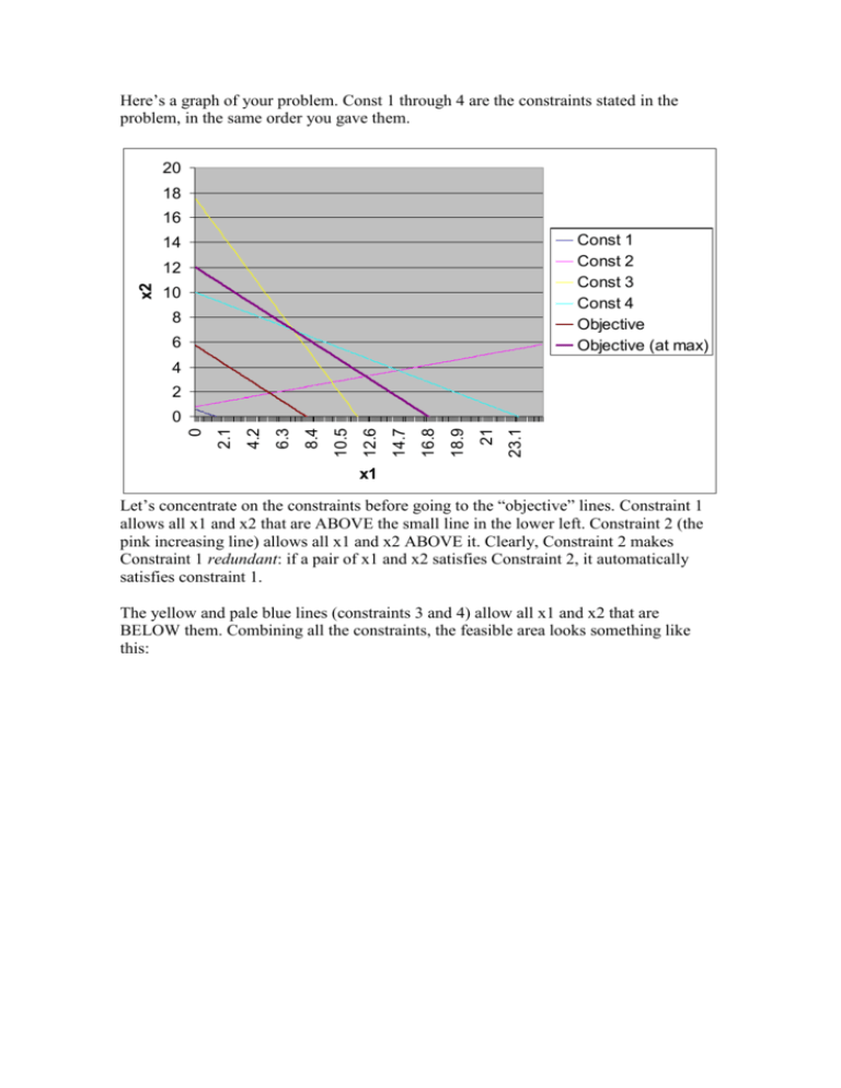
Here’s a graph of your problem. Const 1 through 4 are the constraints stated in the
problem, in the same order you gave them.
20
18
16
Const 1
Const 2
Const 3
Const 4
Objective
Objective (at max)
14
x2
12
10
8
6
4
2
23.1
21
18.9
16.8
14.7
12.6
10.5
8.4
6.3
4.2
2.1
0
0
x1
Let’s concentrate on the constraints before going to the “objective” lines. Constraint 1
allows all x1 and x2 that are ABOVE the small line in the lower left. Constraint 2 (the
pink increasing line) allows all x1 and x2 ABOVE it. Clearly, Constraint 2 makes
Constraint 1 redundant: if a pair of x1 and x2 satisfies Constraint 2, it automatically
satisfies constraint 1.
The yellow and pale blue lines (constraints 3 and 4) allow all x1 and x2 that are
BELOW them. Combining all the constraints, the feasible area looks something like
this:
20
18
16
Const 1
Const 2
Const 3
Const 4
Objective
Objective (at max)
14
x2
12
10
8
6
4
2
23.1
21
18.9
16.8
14.7
12.6
10.5
8.4
6.3
4.2
2.1
0
0
x1
In order to find the solution graphically, the idea is to plot the objective function for an
arbitrary value and then slide to its maximum possible value. Here’s how I did it:
The brown line (called “Objective”) comes from setting 5x1 + 7x2 = 40. The 40 is
arbitrary: this is just an iso-value line, a combination of pairs of (x1, x2) such that the
objective function is 40. (The line formula is obtained easily by isolating x2 from the
5x1 + 7x2 = 40 equation). Now, notice that if we slide this line to the right, we would be
increasing the value of the objective function. Therefore, in order to find the solution,
we just need to keep sliding it to the right until we must stop because we would fall
outside the feasibility area. The “Objective (at max)” line illustrates this: it touches the
feasibility area at just one point. If we sled it a bit more to the right, it would stop
touching the feasibility area, so it would not be a feasible pair of (x1, x2).
We conclude then that the maximum happens at the point we mentioned above: it
coincides with the intersection of constraints 3 and 4. The intersection of these lines
(which can be found using a straightforward system of 2 equations) happens at x1=7
and x2=7. So the maximum is attained at (7, 7).
Ranges of optimality
b. These are the range of values for the coefficients in the objective function such that
the solution would still be (7, 7). They can be found very easily. We can use the
following rules:
- Given an objective function Ax1 + Bx2, the slope of the iso-value line is –A/B
(in this case, it’s -5/7).
- Given a constraint Cx1 + Dx2 = b, the slope of the constraint is –C/D.
Now let’s check the graph once again. If the slope of the objective function was much
steeper, then the solution would stop being located at (7, 7), and would rather be at the
intersection between the Constraints 2 and 3. Likewise, if the slope of the function was
much flatter, then the solution would stop being at (7, 7), and would be located at the
“left” extreme of constraint 4 (you can check all this using the “sliding” procedure with
flatter or steeper objective functions). In fact, the point (7, 7) can only be the maximum
as long as the slope of the objective function is steeper than the slope of constraint 4
AND flatter than constraint 3.
Using the rule I gave you above, we find the slope of constraint 3 is -3/2, and the slope
of constraint 4 is -3/7.
Now, in order to find the range of optimality for the coefficient of x1, we must let this
coefficient vary (let’s call it A) and keep x2’s coefficient constant (at 7). So the slope of
the objective function lines would be –A/7. Combining this with what we found in the
previous paragraphs, we conclude that (7, 7) is the maximum only if:

3
A
3
 
2
7
7
So we have, on one hand:
A
3

7
7
A 3

7 7
A3

And,
3
A
 
2
7
3 A

2 7
21
A
2
So we conclude that the range of optimality for this coefficient is [3, 21/2]. As long as
the coefficient is within this interval, the optimal solution will be at (7, 7).
c. The range of optimality for the coefficient of x2 can be found in a similar fashion.
Let’s set the coefficient of x1 constant at 5, and let’s call B to the coefficient of x2. We
get:
3
5
3
  
2
B
7
So we have, on one hand:
5 3

B 7
35
B
3
And
3
5

2
B
3 5

2 B
10
B
3

So the range of optimality for this coefficient is [10/3, 35/3]
d. If the coefficient of x1 is decreased to 2, the optimum will no longer be at (7, 7),
because 2 is below the range of optimality. The slope of the objective function will
become -2/7. It will be flatter than Constraint 4. Therefore, as we saw before, the
optimum will be located at the “left” extreme of constraint 4. At this point, x1 = 0 and
x2= 10. The optimum is at (0, 10)
e. If the coefficient of x2 is increased to 10, we will still be within its range of
optimality (since 10 is lower than 35/3). Therefore, the optimum will still be at (7, 7)