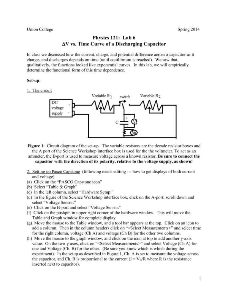
Union College
Spring 2014
Physics 121: Lab 6
V vs. Time Curve of a Discharging Capacitor
In class we discussed how the current, charge, and potential difference across a capacitor as it
charges and discharges depends on time (until equilibrium is reached). We saw that,
qualitatively, the functions looked like exponential curves. In this lab, we will empirically
determine the functional form of this time dependence.
Set-up:
1. The circuit
Figure 1: Circuit diagram of the set-up. The variable resistors are the decade resistor boxes and
the A port of the Science Workshop interface box is used for the the voltmeter. To act as an
ammeter, the B-port is used to measure voltage across a known resistor. Be sure to connect the
capacitor with the direction of its polarity, relative to the voltage supply, as shown!
2. Setting up Pasco Capstone (following needs editing --- how to get displays of both current
and voltage)
(a) Click on the “PASCO Capstone icon”
(b) Select “Table & Graph”
(c) In the left column, select “Hardware Setup.”
(d) In the figure of the Science Workshop interface box, click on the A-port; scroll down and
select “Voltage Sensor.”
(e) Click on the B-port and select “Voltage Sensor.”
(f) Click on the pushpin in upper right corner of the hardware window. This will move the
Table and Graph window for complete display
(g) Move the mouse to the Table window, and a tool bar appears at the top. Click on an icon to
add a column. Then in the column headers click on “<Select Measurements>” and select time
for the right column, voltage (Ch A) and voltage (Ch B) for the other two columns.
(h) Move the mouse to the graph window, and click on the icon at top to add another y-axis
value. On the two-y axes, click on “<Select Measurements>” and select Voltage (Ch A) for
one and Voltage (Ch. B) for the other. (Be sure you know which is which during the
experiment). In the setup as described in Figure 1, Ch. A is set to measure the voltage across
the capacitor, and Ch. B is proportional to the current (I = VB/R where R is the resistance
inserted next to capacitor).
1
Measurements:
1. Set the dials on both variable resistor decade boxes to 3 k. Use a DMM to obtain a more
precise measure of the resistance of both variable resistors. Record these value in the
columns labeled R1 and R2 in the table attached at the back. NOTE: be sure to never let R
get set to zero while discharging the capacitor (step (3))!
2. Charging the capacitor:
(a) First, make sure that the switch is set to connect the capacitor to R2 and wait a few minutes to
be sure that the capacitor is fully discharged.
(b) Without moving the switch yet, turn on the DC voltage supply and set it to 10 volts.
(c) Note the “Record” button on the bottom left. With one partner ready to click “Record” the
other partner moves the switch to connect the capacitor to the voltage supply, and then click
“Record.” Watch the graph and when the capacitor voltage gets sufficiently close to 10 volts,
click “Stop.” Do NOT turn off the voltage supply until the end of the lab.
(d) Move the mouse into the Graph window. A tool bar will appear at the top. Note the icon
that looks like a line fit through a bunch of data, and click on the down arrow next to it.
Throughout this lab, you’ll want to select either “Natural Exponential” or “Inverse
Exponential.”
(e) Find the best-fit curve for both the voltage and the current. Write these best-fit functions in
the columns for Charging in table at the back.
3. Discharging the capacitor:
(a) Get ready to click “Record” again, and move the switch to the right and immediately click
“Record.” Watch the graph and when voltage across the capacitor gets sufficiently close to 0
volts, click “Stop.”
(b) Find the best-fit curve for both the voltage and the current. Write these best-fit functions in
the columns for Discharging in table at the back.
4. Dependence on Resistance:
(a) Change the dial on both resistance boxes to 6k. Use the DMM to record the resistances
and record the values in the second row of the table.
(b) Repeat steps 2 and 3 and record the best-fit functions in the appropriate cells of the table.
Analysis:
1. Compare the general shapes of the I(t) and V(t) curves for charging and discharging for one
set of R’s. Explain these curves in terms of the start and end conditions of the circuit. Include
consideration of whether and when equilibrium occurs in the metal wires as part of your
explanation. Write your answer in the space for question 1 under in the Results table.
2. In this lab, you “charged” and “discharged” the capacitor, but did not measure the “charge” of
the capacitor, because there is no easy way to do so. But, the data can still be used to infer
what Q(t), as a function, looks like. Describe the shape of Q(t) for both charging and
discharging.
3. Compare the rates that I(t) and V(t) change for the different resistances. How does R affect
the rate of charging and discharging? Does R affect both processes similarly?
4. In general, exponents must have no units. Hence, if the exponential describes a function of
time, the factor that is multiplied by time in the exponent must have units of inverse time.
2
The exponential can be re-written as e-t/, where  is called the “time constant.” From your
best-fit functions, determine the time constants for all eight functions and write these values in
Table 2.
5. For charging and discharging capacitors we expect all functions to have a time constant given
by
 = RC.
(a) By manipulating basic circuit equations involving R and C, show that the units of RC is
seconds.
(b) Does the observed dependence on resistance agree?
(c) Calculate the expected time constants in each of your runs by using this equation. Do
these values agree with your data? The capacitance you used is about 10,000 F, or 0.01 F.
3
Results for Lab 6 (Charging and Discharging of a Capacitor)
Name ____________________________ Partner’s Name _____________________________
R1
(kohms)
R2
(kohms)
Table 1: Data Table
V(t) Charging I(t) Charging V(t) Discharging
(volts)
(volts)
(volts)
I(t) Discharging
(volts)
Questions:
1. Compare shapes of V(t) and I(t) for both charging and discharging and explain the similarities
and differences.
2. Sketch what the curve Q(t) for charging would look like? For discharging? Explain, briefly.
3. What is the effect of varying R on the charging and discharging functions?
4
Function
Table 2: Measured and Expected Time Constants
R (kohms)
R (kohms)
expected
measured
expected
measured
V(t)charging
I(t)charging
V(t)discharging
I(t)discharging
5. (a) What are the units of RC?
(b) How well do your ’s agree with the expected values?
(b) Does depend on R as expected?
5