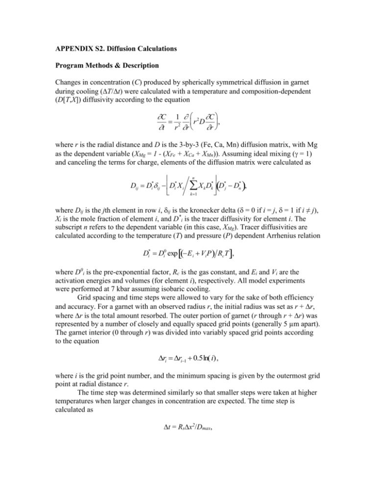
APPENDIX S2. Diffusion Calculations
Program Methods & Description
Changes in concentration (C) produced by spherically symmetrical diffusion in garnet
during cooling (T/t) were calculated with a temperature and composition-dependent
(D[T,X]) diffusivity according to the equation
C 1   2 C 

r D ,
t r 2 r 
r 
where r is the radial distance and D is the 3-by-3 (Fe, Ca, Mn) diffusion matrix, with Mg
as the dependent variable (XMg = 1 - (XFe + XCa + XMn)). Assuming ideal mixing ( = 1)
and canceling the terms 
for charge, elements of the diffusion matrix were calculated as

Dij  Di*ij  Di* X i

 *
*
X
D
 k k D j  Dn* ,

k1
n
where Dij is the jth element in row i, ij is the kronecker delta (= 0 if i = j,  = 1 if i ≠ j),
Xi is the mole fraction of element i, and D*i is the tracer diffusivity for element i. The
 to the dependent variable (in this case, X ). Tracer diffusivities are
subscript n refers
Mg
calculated according to the temperature (T) and pressure (P) dependent Arrhenius relation
Di*  Di0 exp E i  Vi P  RcT ,
where D0i is the pre-exponential factor, Rc is the gas constant, and Ei and Vi are the
activation energies and volumes (for element i), respectively. All model experiments
were performed at 7kbar assuming isobaric cooling.
Grid spacing and time steps were allowed to vary for the sake of both efficiency
and accuracy. For a garnet with an observed radius r, the initial radius was set as r + r,
where r is the total amount resorbed. The outer portion of garnet (r through r + r) was
represented by a number of closely and equally spaced grid points (generally 5 µm apart).
The garnet interior (0 through r) was divided into variably spaced grid points according
to the equation
ri  ri1  0.5ln( i) ,
where i is the grid point number, and the minimum spacing is given by the outermost grid
point at radial distance r.
The time step wasdetermined similarly so that smaller steps were taken at higher
temperatures when larger changes in concentration are expected. The time step is
calculated as
t = Rsx2/Dmax,
where x is the minimum grid spacing, Dmax is the maximum element of the diffusion
matrix (at temperature T using the garnet core composition), and Rs (< 0.5) is a stability
constant (see Crank, 1975, pg. 144).
Program sequence

0. Calculate D(T,X) and Dmax using the core composition and the starting T.
1. Calculate the time step as t = Rsx2/Dmax where Dmax is the largest component of
the D matrix. Check to see whether the cooling rate (CR) has changed.
2. Calculate the new temperature as T = T - T, where T = CR*t.
3. Determine the rim composition and garnet radius corresponding to the new
temperature (T-X-r relations from Program Gibbs, Table S1). If the amount of
resorbtion exceeds the outer grid spacing, then the outermost grid point is
removed. The new rim composition at the current temperature is set to the
outermost grid point. Since Gibbs compositions were used, no mass balance was
performed (these values should reflect the necessary compositional changes at the
rim).
4. Calculate r 2 DC r for each grid point. The gradient, C r , at each interior grid
point is calculated as Ci1  Ci1  /r (i refers to the grid point) and matrixmultiplied by the 3-by-3 diffusion matrix and the scalar r2. The gradient of the
core
is zero. Dmax is recalculated here and stored for later.


5. Calculate the change in concentration as C = C + C. If A  r 2 D C r , then

C  Ai1  Ai1t /r 2r for each interior grid point. The change in rim
composition has been set previously (step 3) and is not calculated here. The core
2
composition is calculated as C  6Dt C2  C
1/r (see Crank, 1975, eqn. 8.39,
pg. 149). Finally, XMg is calculated for each grid point as 1 - (XFe + XCa + XMn)
and the sequence continues at step 1.
Other Considerations

The peak Ca concentration profile is an unknown since it depends on the prograde P-T
path. However, the variation in Grs is minor and has little to no effect on the resulting
FM and Sps profiles. Observed profiles were shifted up or down as necessary to align
them with the model profiles.