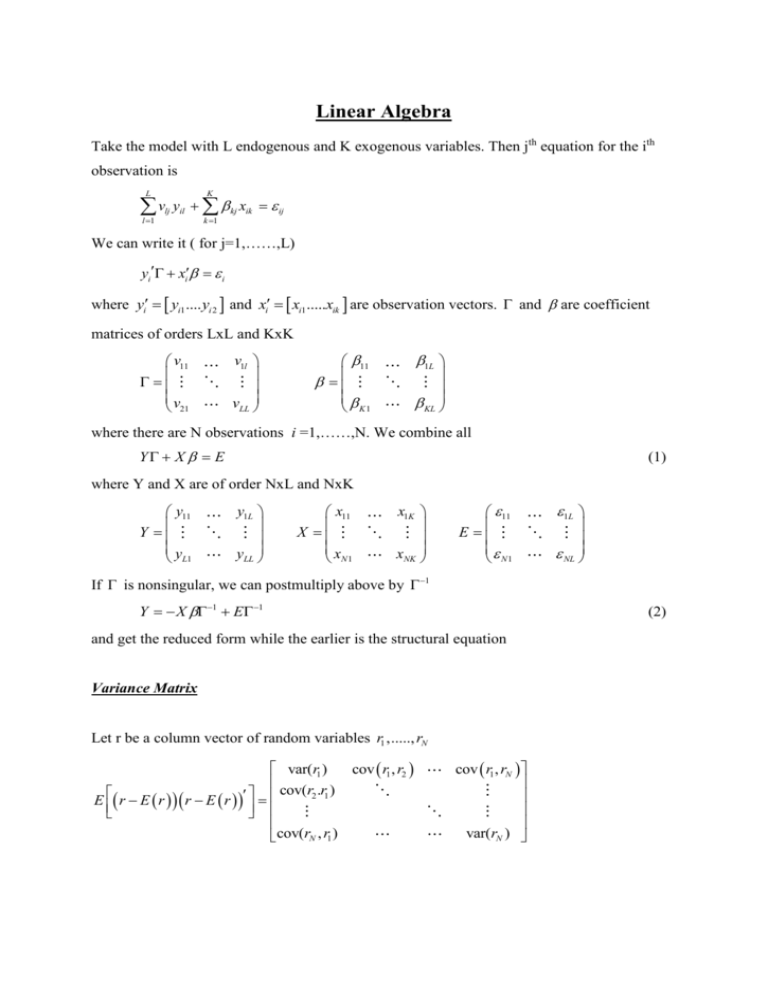
Linear Algebra
Take the model with L endogenous and K exogenous variables. Then jth equation for the ith
observation is
L
K
l 1
k 1
 vlj yil    kj xik   ij
We can write it ( for j=1,……,L)
yi  xi   i
where yi   yi1 .... yi 2  and xi   xi1 .....xik  are observation vectors.  and  are coefficient
matrices of orders LxL and KxK
 v11


v
 21
v1l 


vLL 
 11
  

 K1
1L 


 KL 
where there are N observations i =1,……,N. We combine all
Y  X   E
(1)
where Y and X are of order NxL and NxK
 y11

Y 
y
 L1
y1L 


yLL 
 x11

X 
x
 N1
x1K 


xNK 
 11

E 

 N1
1L 


 NL 
If  is nonsingular, we can postmultiply above by  1
Y   X 1  E 1
(2)
and get the reduced form while the earlier is the structural equation
Variance Matrix
Let r be a column vector of random variables r1 ,....., rN
 var(r1 )
cov  r1 , r2 

cov(r2 .r1 )


E  r  E  r    r  E  r     

 

cov(rN , r1 )
cov  r1 , rN  




var(rN ) 
Least Squares
y  x  
b   x x  x y
1
(3)
because ee  y y  2 y xb  bx xb is minimized by changing b.
b     x x  x 
1
if E    is 0 and x is nonrandom, then b is unbiased.
var(b)   x x  x  var    x  x x    2  x x 
1
1
1
since var     2  . Substitution of (3) into e  y  xb yields the protection matrix e  My ,
where M is symmetric and idempotent.
M  I  X  X X  X 
1
since MX=0, e  My  M  x      M  . Also M 2 =M, causing the residual sum of squares
ee   M M    M 2 
ee   M 
Trace:
The trace of a square matrix is the sum of its diagonal elements
tr(AB) = tr(BA) if both exist
tr(A+B) = tr(A)+tr(B) if they are of same order
example:
E  ee   E   M    trE  M   
= tr E      trX   X X  XE    
1
  2 tr      2 tr  X X  X X
1
  2n   2k
  2 n  k 
Generalized Least Squares
If cov     2 v rather than  2  where v is nonsingular then
ˆ   xv 1 x  xv 1 y
1
and
 
1
var ˆ   2  x v 1 x 
(derived later in Aitken`s Theorem)
Partitioned matrices:
Take the system in (2) and rewrite it as Y  Y1Y2 
 y13 y12 

Y2  

 yn3 yn 2 
 y11 y12 

Y1  

 yn1 yn 2 
We partition by sets of columns.
Rules:
 A11
A
 21
A12   B11

A22   B21
B12   A11  B11

B22   A21  B21
 A11 B11  A12  B21
 A21 B11  A22 B21
 A B  
A12  B12 
A22  B22 
A11 B12  A12 B22 
A21 B12  A22 B22 
Inverse of a symmetric partitioned matrix:
1
 D

 DBC 1
A B

 1
 B C 
1
1
1 


 C BD C  C BDBC 
 A1  A1BEBA1  A1BE 
=

 EBA1
E 

where D   A  BC 1 B   and E   C  B A1 B  . We use the first when C is nonsingular and
1
second when A is nonsingular.
Application: deviation from mean
i i
 x i

ix 
x x 
bottom right of inverse
 X MX 
1
1
M    ii 
n
Kronecker Product
A special form of partitioning when all submatrices are scalar multiples of the same matrix.
 a11 B
A  B  
 am1 B
a1n B 


amn B 
We refer to this as Kronecker product of A and B. If B is pxq, then the order is mpxnq
 A  B    C  D   AC  BD
1
 A  B   A1  B 1 since  A  B   A1  B 1   AA1  BB 1
 A  B   A1  B 1
A   B  C    A  B   A  C 
 B  C   A   B  A   C  A
1
Application: Joint GLS
yj  xj  j   j
 X1 0
 y1  
  0
  
 y2  
 0
j=1,......,L for L endogenous variable
0
0  1   1 
   
    
0    
   
X L 
  L    L 
Y  Z 
If we assume n disturbances of L equations have equal variance and uncorrelated so that
var( j )   jj I and for j  i E ( j i ) contains contemporaneous covariances, then the full
covariance matrix
 11 I  12 I
 I  I
22
var( )   21


 L1 I
 1L I 

   I


 LL I 
where
Assuming  is non-singular, application of GLS results in
ˆ  ( Z ( 1  I ) Z ) 1 Z ( 1 I ) y
and
var(ˆ )   Z (1 I ) Z 
1
̂ is superior to Least Squares unless X i are all identical causing
  
j1

X
0
Z 


0
0
X
0
0

IX
0

X
Z ( 1  I ) Z )  ( I  X )( 1  I )( I  X )   1  ( X X )
var GLS
var OLS
or  is diagonal, indicating no covariance between j and i.
Vectorization
Sometimes we need to work with vectors rather than matrices, e.g. finding the variance of
 k . If the  ’s are in a matrix form B. Therefore, we vectorize these parameters by:
A=  a1 .........aq  (a pxq matrix), ai being the i’th column of A.
vec(A) =  a1 a2
aq  which is a pq element column vector.
vec(A+B) = vec(A)+vec(B)
vec(AB)= ( I  A)vec( B)  ( B   I )vec( A)
Definiteness
If the quadratic form xAx is positive for any x  0 is said to be positive definite. The
covariance matrix  of any random vector is always positive semi definite.
Example: BLUE implies Var (  )  var(b) is positive semi definite.
Proof:  is linear in y so =  y . Define C = B - ( X X ) X 
To write  y as
C  ( X X ) 1 X  y  C  ( X X ) 1 X   X    
=(CX  I )  + C  ( X X )1 X  
Unbiasedness implies CX = 0.
var(  )  C  ( X X ) 1 X  var( ) C  ( X X ) 1 X 
= 2CC    2 ( X X ) 1   2 CX ( X X ) 1   2 ( X X ) 1 X C 
0
0
The difference  2 CC  is positive semi definite because  2 wCC w  ( C w)( Cw) is the
non-negative squared length of the vector  Cw (inner product). We use definiteness in
evaluation of minima and maxima; e.g. for maximizatior of utility the Hessian should be
negative definite. If a matrix is definite and black diagonal, the principal submatrices are also
definite.
Diagonalization
For some nxn matrix A, we seek a vector x so that Ax equals  x (  is a scalar) This is
trivially satisfied by x = 0 so we impose xx  1 implying x  0 .
Ax   x  ( A   I ) x  0,
xx  1
(4)
 A   I is singular
 A   I  0 (characteristic equation)
If A is diagonal, then the terms in the diagonal will be the solution to the characteristic eq.
The determinant is a polynomial of degree n and has i as the latent roots. The product of i
equals the determinant of A, and the sum i equals the trace of A. All vectors are called
characteristic (eigen)vectors.
If A is symmetric x Ay  y Ax , so assume i and  j are two different roots with vectors xi
and x j .
Premultiplying Axi  i xi by x j and Ax j by xi and then subtract
x j Axi  xiAx j  (i   j ) xix j
For a symmetric matrix, left side vanishes and (i   j ) is non zero, implying orthogonality of
the characteristic vectors.
X X  I
where X   x1 x 2 ......xn 
AX=  Ax1 Ax 2 .....Ax n   1 x1.......n xn 
AX  X 
where  is diagonal with i on the diagonal. Premultiply by X 
X AX  X X   
This double multiplication diagonalizes A (symmetric). Also postmultiplication
n
AXX   A  X X    i X i X i
i 1
Special cases: If A is square Ax   x
A2 x   Ax   2 x
which shows that the roots of a square matrix A2 is the square of  . For symmetric and non
singular A premultiply both sides by ( A) 1 to obtain
A1 x 
1

x
All latent roots of a positive definite matrix are positive.
Aitken’s theorem:
Any symmetric positive definite matrix A can be written as A  QQ  where Q is some nonsingular matrix. For example, consider the covariance matrix  2V . This matrix is positive
def. So its inverse also is. So we can decompose it V 1  QQ . We premultiply both sides of
y  X 
by Q
Qy  (Q X )   Q 
   (QX )(QX ) (Q X )Q y  ( X QQ X ) 1 X QQy
1
 ( X V 1 X )1 X V 1 y
(GLS)
var( Q)   2 QVQ   2 Q(QQ)1 Q   2 QQ 1Q 1Q   2 I
Cholesky decomposition
Rather than using an orthogonal matrix, X, in the previous diagonalization, it is also possible
to use a triangular matrix. For instance, consider a diagonal D and an upper triangular C with
units in the diagonal.
1 C12
C  0 1
0 0
C13 
C23 
1 
 d1 0
D   0 d 2
 0 0
0
0 
d3 
yielding
 d1
C DC   d1c12
 d1c13
d1c12
d c  d2
d1c12c13  d 2c23
2
1 12

d1c12c13  d 2c23 
2
d1c132  d 2c23
 d3 
d1c13
Any symmetric positive definite matrix A   aij  can be uniquely written as CDC
(d1  a11 , c12  a12 a11 , etc.) , which is referred to as the Cholesky decomposition.
Simultaneous diagonalization of two matrices
( A   B) x  0
xBx  1
(5)
where A and B are symmetric nxn matrices, is being positive definite. B1 is also positive def.
So B 1  QQ .
(QAQ   I ) y  0
yy  1
y  Q-1 x
This shows that (5) can be reduced to (4) when A in (4) is interpreted as Q AQ . If A is
symmetric, so is Q AQ . (5) has n solutions 1 ...........n , and if they are distinct, then X i are
unique.
( A   B) x  0 as
Axi   Bxi
and
AX  BX 
premultiplication by X 
X AX  X BX   
Therefore
X AX   and X BX  I
which shows that matrices being diagonalized together, A into the latent root matrix and B
into I.
Example: Constrained extremum
Maximize xAx subject to xBx  1 with respect to x
Lagrangian  x AX   ( x Bx  1)
L
 2 Ax  2  Bx  Ax   Bx
x
which shows that  must be a root. Next premultiply by x   x Ax   x Bx   shows that
the largest root i is the maximum of xAx st xBx  1
Principal components
Consider nxk observation matrix Z. The objective is to approximate Z by a matrix of unit
rank, vc , where V is an n element vector and C is a k element coefficient vector. The
objective is to minimize the discrepancy matrix Z  vc by minimizing the square of all KN
discrepancies and also impose vv  1 to be able to solve for c. The solution when v  v1 and
c  c1 is
( ZZ   1 I )v1  0
c1  Z v1
So 1 is the largest latent root of ZZ  . Next to approximate Z by v1c1  v2 c2 , we again
minimize the discrepancies st. v2 v2  1 and v2 v1  0 . The solution again is
( ZZ   2 I )v2  0
c2  Z v2
which is the second largest root and the corresponding vector. You can generalize to i roots.
Derivation for 1 root
Since the sum of squares of any matrix A is equal to trace AA , the discrepancy matrix sum of
squares is
tr  Z  vc   Z  vc   trZ Z  trcvZ  trZ vc  trcvvc
inner products since c=vZ
trZ Z  2v Zc   v v  c c 
 trZ Z  2v Zc  c c
Derivative wrt c is 2Z v  2c  c  Z v
Substituting this back in, we get trZ Z  vZZ v , so to minimize the discrepancy, maximize
vZZ v wrt v st vv  1
Langrangian  vZZ v    vv 1
ZZ v   v  v ZZ v   v v  
This, shows that the maximum root,  , minimizes ZZ  . Extend to i cases.
Z Z need not be diagonal; the observed variables can be correlated. But the principle
components are all uncorrelated because vj v j  0 for i  j . Therefore, these components can
be viewed as “uncorrelated linear combinations of correlated variables”.