SPLUS SIMULATION EXAMPLES
INVERSE CDF METHOD
The following function – called ran.exp – produces a random sample of size n
from an exponential distribution with parameter b>0. It uses the inverse CDF
method.
SIMULATING n EXPONENTIAL VARIATES WITH PARAMETER BETA=b
ran.exp<-function(n, b=1){
u<-runif(n)
x<- -log(1-u)/b
x}
To run it in R, type:
X<-ran.exp(100,5)
This will produce a vector x containing the random sample (size=100,
parameter=5)
To produce a histogram, type:
hist(x)
REJECTION METHOD
The following function – called norm.rej – produces a random sample of size n
from a normal distribution with mean m and standard deviation s>0. It uses the
rejection method (where g is the Laplace PDF).
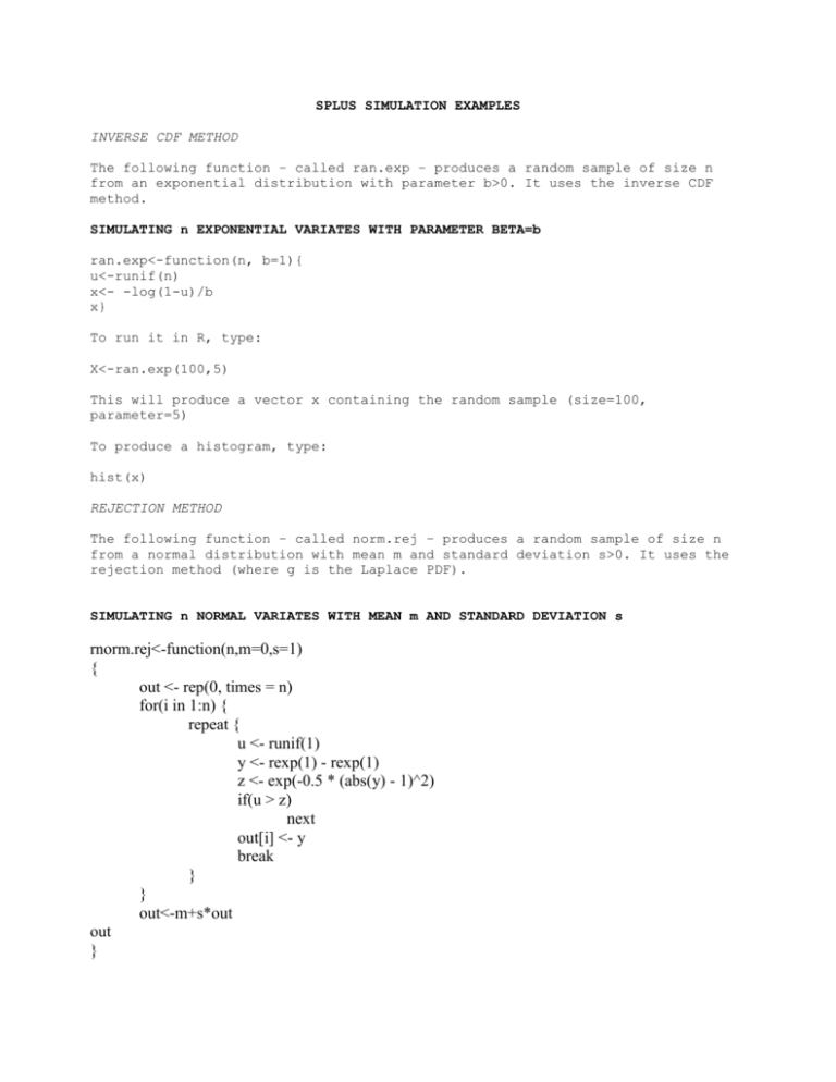
SIMULATING n NORMAL VARIATES WITH MEAN m AND STANDARD DEVIATION s
rnorm.rej<-function(n,m=0,s=1)
{
out <- rep(0, times = n)
for(i in 1:n) {
repeat {
u <- runif(1)
y <- rexp(1) - rexp(1)
z <- exp(-0.5 * (abs(y) - 1)^2)
if(u > z)
next
out[i] <- y
break
}
}
out<-m+s*out
out
}
To run it in R, type:
X<-norm.rej(100,0,1)
This will produce a vector x containing the random sample (size=100, standard
normal)
To produce a histogram, type:
hist(x)
ILLUSTRATIONS OF LLN
The following R function provides a plot of k versus S(k)/k, k=1, 2, 3, …, n, where S(k) is the sum
of the first k values of a sequence of IID exponential random variables with parameter b.
lln.exp.example<-function(n,b=1){
x<-ran.exp(n,b)
y<-1:n
for (i in 1:n){
y[i]<-mean(x[1:i])
}
plot(1:n,y)}
The following R function provides a plot of k versus S(k)/k, k=1, 2, 3, …, n, where S(k) is the sum
of the first k values of a sequence of IID Cauchy random variables with scale parameter b.
lln.cauchy.example<-function(n,b=1){
x<-rnorm(n)/rnorm(n)
x<-b*x
y<-1:n
for (i in 1:n){
y[i]<-mean(x[1:i])
}
plot(1:n,y)}
ILLUSTRATIONS OF SUM AND RANDOM SUM/CLT FOR STANDARD
EXPONENTIAL DISTRIBUTION
The following R function produces k IID copies of the random sum (with geometric number of
terms N) of IID standard exponential random variables. The mean of N is 1/p.
ran.sum.exp.illustration<-function(k, p){
v<-1:k
for (i in 1:k){
n<-rgeom(1,prob=p)+1
v[i]<-sum(rexp(n))}
v}
In contrast, the following R function produces k IID copies of a deterministic sum (with fixed n
terms) of IID standard exponential random variables.
sum.exp.illustration<-function(k, n){
v<-1:k
for (i in 1:k){
v[i]<-sum(rexp(n))}
v}
The empirical distributions obtained by these two functions are quite different!
The following R function produces k IID copies of the (normalized) sample mean of size n from
standard exponential distribution.
clt.exp.illustration<-function(k, n){
v<-1:k
for (i in 1:k){
v[i]<-sqrt(n)*(mean(rexp(n))-1)}
v}