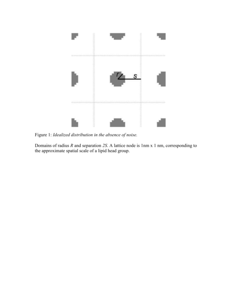
Figure 1: Idealized distribution in the absence of noise.
Domains of radius R and separation 2S. A lattice node is 1nm x 1 nm, corresponding to
the approximate spatial scale of a lipid head group.
A
B
Figure 2: Different FRET methods.
A) Intra-domain FRET
B) Segregation FRET I, donors within domains
C) Segregation FRET II, donors outside domains
C
A
B
C
Figure 3: Segregation FRET (Donors within Domains) and Approximations.
A) Local Acceptor Neighborhood of a Random Donor
B) FRET Efficiency decreases with domain radius and increases with Forster length
with analytic estimates (fits s = …)
C) FRET Efficiency decreases with domain radius and increases with acceptor
density with analytic estimates (fits s = …)
D) Simulated FRET Efficiency, Analytic Solution and Analytic Estimate when s=0
E) plots of s verses forster length and acceptor density
A
B
C
Figure ?: Ripley’s K
Comparison of second-order measures for an aggregated point distribution (solid line)
and a random (Poisson) distribution (dotted line). A) Ripley’s K function, B) L function
C) H function and D) M function. Points of aggregated distributions are randomly
dispersed within disks of radius R and separation 2S. Curves for aggregated distributions
show the mean and standard deviation of 10 independent distributions.
A
B
C
D
E
F
Figure 4: Investigation Methods in the case of Idealized Domains.
A)
B)
C)
D)
E)
F)
Intra-domain FRET measures intra-domain density
With calibration, Intra-domain FRET measures domain fraction
With calibration, segregation fret I measures domain radius
K function predicts domain radius
L function predicts domain radius
but H does not since H max depends on both R and S
By calibration, I mean that the FRET efficiency doesn’t translate directly to the domain
radius or domain separation, you need to know the dependence of E verses domain radius
/ domain separation in advance.
Figure 5: Comparing domain measures for a compact verses elongated shapes.
A) Intra-domain FRET is robust to elongation. Only in the case of quasi-1-dimensional
objects it’s somewhat reduced.
B) Ripley’s measures the domain radius along its widest dimension and segregation
FRET measures the domain radius along its shortest dimension.
C) For disks, Ripley’s K and segregation FRET measure the domain radius as already
shown. For stripes, Ripley’s K measures the stripe length (not terribly meaningful) while
segregation FRET measures the stripe half-width (what we’re interested in). For this
figure, we increase the stripe width while keeping the stripe length constant: Ripley’s K
prediction is constant but seg FRET increases proportional to stripe width.
Figure 6: Comparing domain measures for a smooth verses rough domain boundaries.
A) smooth verse rough domain edge can be parametrized by the length of the
protrusions stuck out and stuck in
B) Intra-domain FRET is robust to domain edge noise. Only in the case of quasi-1dimensional disk (perturbations are so great the shape is quasi-linear/fractal as
shown) it’s somewhat reduced.
C) Ripley’s K is robust to domain edge perturbation (the predicted radius is inflated
only by the perturbation length) but segregation FRET is decimated since it
measures the half-width of the protrusions instead of the half-width of the domain
Figure 7: Comparing measures in the context of random thinning.
A) Self-FRET yields the actual domain fraction with the most accuracy when the
acceptor density is high (red points) verses when the acceptor density is low
(black points).
B) Segregation FRET is perfectly robust to thinning of the donor density within
domains, thinning of the acceptor density outside domains results in a lower
FRET efficiency and a more shallow slope of the dependence upon domain radius
(less sensitivity).
C) Ripley’s K is robust to thinning, but at extremely low density tends to underestimate the domain radius and have larger error bars.
Figure 8: Measures in the context of random holes in the pattern.
All measures are fairly robust to the random seeding of large proteins and other domain
types.
A
B
C
Figure 8: Comparing Domain Measures in the context of variation in domain separation
that is small compared to the domain radius (i.e., domain interaction).
A) The extent of domain overlap makes no difference to intra-domain FRET (solid
line) and little difference to segregation FRET (dotted line).
B) Closely spaced domains causes Ripley’s K to predict two spatial scales of
clustering and a single larger scale of clustering for overlapping domains.
Figure 9: Comparing effect of noise in domain organization (monomer fraction).
A) Intra-domain FRET
a. Error bars show mean and std FRET efficiency verses density of
monomers outside domains.
b. Dotted line shows FRET efficiency if only contribution of transfers and
decays of donors within domains is considered.
c. Dashed line shows FRET efficiency if only contribution of transfers and
decays of donors outside domains is considered.
B) Segregation FRET
a. Error bars show mean and std FRET efficiency verses density of
monomers outside domains.
b. Dotted line shows FRET efficiency if only contribution of transfers and
decays of donors within domains is considered.
c. Dashed line shows FRET efficiency if only contribution of transfers and
decays of donors outside domains is considered.
C) Ripley’s K – very robust to a small monomer fraction.
Intra-domain FRET and Segregation FRET are sensitive to the monomer fraction, and the
extent of error scales with the ratio of the monomer fraction to the domain fraction.
Ripley’s K is wholly immune.
III. Domain Investigation Methods applied to an example. (Figures 8 – 11)
A
B
C
D
E
F
Figure 10: Lipid Partitioning Model
Separation of raft and non-raft lipids results in domain formation. The relative fraction of
raft (blue pixels) and non-raft lipid (yellow pixels) is .25 and .75. Interaction energies are
chosen so that the raft lipids (LR) phase separate from the non-raft (LNR) lipids: LRLR =
LNRLNR = 0, LRLNR =1. The distribution of lipids at time step (A) 0, (B) 100 and (C)
1000. (D) Mean lattice energy per lattice node over time. (E) Average domain area over
time. (F) Average domain area at 2000 time-steps verses temperature K. Error bars show
mean and standard deviation of 5 simulations.
Figure 11: Varying the domain fraction, number of time steps.
Domains of raft (blue) and non-raft (yellow) lipids when interaction energies are chosen
so that the raft lipids (LR) phase separate from the non-raft (LNR) lipids: LRLR =
LNRLNR = 0, LRLNR =1. The temperature K=3. Left to right: Increasing the fraction of
raft lipid increases the total area of raft domains. Raft lipid fractions are 0.1, 0.3, 0.5, 0.7
and 0.9. Top to bottom: Increasing the number of time steps increases the area of each raft
domain before the percolation transition and increases the area of each non-raft domain
before the percolation transition. For 200, 2,000 and 10,000 time steps.
Figure 12: Naïve measures of domain size.
A) Mean domain area (as number of lipids) verses domain fraction.
B) Mean domain width (as number of lipid diameters) verses domain fraction.
C) Total domain perimeter divided by total domain area verses domain fraction.
Red, black and blue lines show measures for patterns after 200, 2000 and 10,000 time
steps. Error bars indicate the standard deviation of means for patterns after 2000 time
steps.
Figure 13: Generating calibration curve for segregation FRET.
Intra-domain FRET
Segregation FRET
Ripley’s K
Use Ripley’s K to plot
predicted domain width
verses actual domain
width. Probably only
works far from the
percolation threshold.
Will use previous figure to
deduce domain width, then
plot predicted domain width
verses actual domain width.
Seems pretty overwhelmed by
noise .. mainly due to the
variation in domain radius
being too large compared to
domain separations
(remember, the domain radius
is measured along the longest
dimension and small
separations are treated as
holes in the pattern and
ignored)
Figure 14: Applications for irregular domains generated by lipid partitioning model
A-C) Raw data for the different methods.
D-F) Applications of the data for the different methods. Predicting domain fraction,
domain width and domain separation.
Can discuss the effect of increasing time/decreasing noise.
Some Conclusions
Intra-domain FRET is exceptionally robust as a predictor of the local acceptor density
and domain fraction. Segregation works very well in the model for domain formation
we’ve considered. Although it requires calibration, it was calibrated on domains before
the percolation transition and worked equally well before and after.
FRET methods try to solve the inverse problem, while Ripley’s K is a statistic on a given
distribution (forward problem). There are other statistics than can be used – average peak
interval method, for example, is robust to elongation, where Ripley fails.