IE312
HW#7 Solution
1 of 5
1. Chapter 9 Problem 19
Notations:
Yi = 1 if Hallo decide to run shift i, and = 0 otherwise (i = 1, 2, 3, 4)
Xi = amount produced in shift I, (i = 1, 2, 3, 4)
 1 for day 1
 2 for night 1

i
 3 for day 2
4 for night 2
Decision variables: Yi, Xi
Objective function:
Min Z = Setup Cost + Inventory Cost
Where
Setup Cost = 8000(Y1+Y3)+ 4500(Y2+Y4)
Inventory Cost = (X1-2000)+( X1+ X2-5000)+( X1+ X2+ X3-7000)+( X1+ X2+ X3+ X4-10000)
Constraints:
1) Demand Constraints
X12000
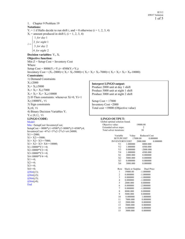
Interpret LINGO output:
X1+ X25000
Produce 2000 unit at day 1 shift
X1+ X2+ X37000
Produce 5000 unit at night 1 shift
X1+ X2+ X3+ X410000
Produce 3000 unit at night 2 shift
2) If-Then constraints: whenever Xi>0, Yi=1
Xi≤10000Yi, i
Setup Cost = 17000
3) Sign constraints
Inventory Cost =2000
Total cost =19000 (Objective value)
Xi0, i
4) Binary Decision Variables Yi
Yi{0,1}, i
LINGO CODE:
LINGO OUTPUT:
Model:
Min =SetupCost+InventoryCost;
SetupCost = 8000*y1+4500*y2+8000*y3+4500*y4;
InventoryCost =4*x1+3*x2+2*x3+x4-24000;
X1>=2000;
X1+ X2>=5000;
X1+ X2+ X3>=7000;
X1+ X2+ X3+ X4>=10000;
X1-10000*Y1<=0;
X2-10000*Y2<=0;
X3-10000*Y3<=0;
X4-10000*Y4<=0;
X1>=0;
X2>=0;
X3>=0;
X4>=0;
@bin(y1);
@bin(y2);
@bin(y3);
@bin(y4);
End
Global optimal solution found.
Objective value:
Extended solver steps:
Total solver iterations:
19000.00
2
38
Variable
Value
Reduced Cost
SETUPCOST
17000.00
0.000000
INVENTORYCOST
2000.000
0.000000
Y1
1.000000
8000.000
Y2
1.000000
4500.000
Y3
0.000000
-2000.000
Y4
1.000000
4500.000
X1
2000.000
0.000000
X2
5000.000
0.000000
X3
0.000000
0.000000
X4
3000.000
0.000000
Row Slack or Surplus
Dual Price
1
19000.00
-1.000000
2
0.000000
-1.000000
3
0.000000
-1.000000
4
0.000000
-1.000000
5
2000.000
0.000000
6
0.000000
-2.000000
7
0.000000
-1.000000
8
8000.000
0.000000
9
5000.000
0.000000
10
0.000000
1.000000
11
7000.000
0.000000
12
2000.000
0.000000
13
5000.000
0.000000
14
0.000000
0.000000
15
3000.000
0.000000
IE312
HW#7 Solution
2 of 5
2. Chapter 9 Problem 20
Same Notations and Decision Variables as #1
Objective function:
Min Z = Setup Cost + Inventory Cost
Where
Setup Cost = 1000(Y1+Y3)+ 3500(Y2+Y4)
Inventory Cost = (X1-2000)+( X1+ X2-5000)+( X1+ X2+ X3-7000)+( X1+ X2+ X3+ X4-10000)
Same Constraints as #1
LINGO CODE:
Model:
Min =SetupCost+InventoryCost;
SetupCost = 1000*y1+3500*y2+1000*y3+3500*y4;
InventoryCost =4*x1+3*x2+2*x3+x4-24000;
X1>=2000;
X1+ X2>=5000;
X1+ X2+ X3>=7000;
X1+ X2+ X3+ X4>=10000;
X1-10000*Y1<=0;
X2-10000*Y2<=0;
X3-10000*Y3<=0;
X4-10000*Y4<=0;
X1>=0;
X2>=0;
X3>=0;
X4>=0;
@bin(y1);
@bin(y2);
@bin(y3);
@bin(y4);
End
LINGO OUTPUT:
Global optimal solution found.
Objective value:
Extended solver steps:
Total solver iterations:
Interpret LINGO output:
Produce 5000 unit at day 1 shift
Produce 5000 unit at day 2 shift
Setup Cost = 2000< 17000 (Setup Cost form #1)
Inventory Cost =6000 > 2000 (Inventory Cost form #1)
Total cost =8000 (Objective value)
Compared result to #1
We see that the setup cost decreases while the inventory cost
increases  The decrease in setup costs has actually raised
the average inventory level!
8000.000
3
24
Variable
Value
Reduced Cost
SETUPCOST
2000.000
0.000000
INVENTORYCOST
6000.000
0.000000
Y1
1.000000
1000.000
Y2
0.000000
-6500.000
Y3
1.000000
1000.000
Y4
0.000000
-6500.000
X1
5000.000
0.000000
X2
0.000000
0.000000
X3
5000.000
0.000000
X4
0.000000
0.000000
Row Slack or Surplus
Dual Price
1
8000.000
-1.000000
2
0.000000
-1.000000
3
0.000000
-1.000000
4
3000.000
0.000000
5
0.000000
-2.000000
6
3000.000
0.000000
7
0.000000
-2.000000
8
5000.000
0.000000
9
0.000000
1.000000
10
5000.000
0.000000
11
0.000000
1.000000
12
5000.000
0.000000
13
0.000000
0.000000
14
5000.000
0.000000
15
0.000000
0.000000
IE312
HW#7 Solution
3 of 5
3.
Chapter 9 Problem 22
“A job cannot be processed on machine j unless for all i<j the job has completed its processing on machine i.
once a job begins its processing on machine j, the job cannot be preempted on machine j.”
From above constraint, we know that job 1 has to be produced at M/C 1 first, and then M/C 3, and finally M/C
4, job 2 has to be produced at M/C 1 first, and then M/C 2, and finally M/C 4, and job 3 has to be produced at
M/C 2 first, and finally M/C 3. A summarize of machine order and the processing time for all job are shown
below.
Job
Machine Order
Processing time
1
1-3-4
P11=20. P31=25, P41=30
2
1-2-4
P12=15, P22=20, P42=18
3
2-3
P23=35, P33=28
Notations:
Pij is the processing of job j at machine i, i= 1.2.3.4 and j=1, 2, 3
Yij = Production starting time of job j at machine i
Fj = Flow time of job j
Note that
Flow Time of job j= Production Completion Time of job j at the last M/C the job has been produced–
Production Starting time of job j at the first M/C the job has been produced, and
Production Completion Time of job j at the last M/C the job has been produced = Production Starting Time of
job j at the last M/C the job has been produced + Processing time at the last M/C of the job
Decision variables: Yij
Objective function:
3
Min
F
j 1
j
/3
Where
F1  Y41  30  Y11
F2  Y42  18  Y12
F3  Y33  28  Y23
Constraints:
1) Type 1 Constraints
Y31  Y11  20
Y41  Y31  25
Y22 Y12  15
Y42 Y22  20
Y33 Y23  35
2) Type 2 Constraints
Y11 Y12  15 or
Y22  Y23  35 or
Y31  Y33  28 or
Y41 Y42  18 or
3) Sign Constrains
Fj,Yij 0, i,j
Y12 Y11  20
Y23 Y22  20
Y33  Y31  25
Y42 Y41  30
IE312
HW#7 Solution
4 of 5
4.
Chapter 14 Problem 5
Simulated Annealing (SA) for a single-machine scheduling problem with minimizing tardiness
Notation:
S0 is the best schedule found so far
(k )
(k )
(k )
(k )
(k )
(k )
Sk is the current schedule, Sk = ( j1 , j 2 ,, ji 1 , ji , ji 1 ,, j n )
G(Sk) is the tardiness of a schedule
Sc is the candidate schedule
Aspiration Criterion: G(Sk)  G(S0)
Acceptance Criterion: If G(Sc) < G(Sk), accept Sc and let Sk+1 = Sc
If G(Sc)  G(Sk), move to Sc with probability P(Sk+1, Sc) = ec/  k
c = G(Sk) - G(Sc)
Step 1:
Set k=1 and select the initial temperature 1,
To choose initial temperature 1 for Simulated Annealing, we will start with the 1 large number that later will
be slowly lowered in cooling steps. The value of 1 depends on maximum possible tardiness (worst schedule).
n
The worst case of the schedule is when all due date (dj) is equal to 0. We have 1=
P

j 1
j
Pj = Processing time of job j
(1)
(1)
(1)
(1)
(1)
(1)
Select an initial schedule S1 and set S0=S1= ( j1 , j 2 ,, ji 1 , ji , ji 1 ,, j n )
Step 2:
Select a candidate schedule Sc from N(Sk).
How to select a candidate depends on neighborhood structure.
Let us considered random pairwise job interchange as a type of schedule generation schemes. The schedule is
generated by randomly selecting any pair of distinct jobs within the schedule and exchanging their position.
(k )
(k )
(k )
(k )
(k )
(k )
Since Sk = ( j1 , j 2 ,, ji 1 , ji , ji 1 ,, j n ) , when exchanging position i with position i+1
(k )
(k )
(k )
(k )
(k )
(k )
we will have Sc = ( j1 , j 2 ,, ji 1 , ji 1 , ji ,, j n )
If G(S0)< G(Sc) < G(Sk), set Sk+1 = Sc and go to step 3
If G(Sc)< G(S0), set S0 =Sk+1 = Sc and go to step 3
If G(Sc) < G(S0), generate Uk~Uniform(0,1);
If Uk≤P(Sk, Sc), set Sk+1 = Sc; otherwise set Sk+1 = Sk; go to step 3
Step 3:
Select k+1≤k,
Let k = k+1, if k= N STOP; otherwise go to Step 2.
Note that as k decreases, the lower the probability to accept worse schedules.
IE312
HW#7 Solution
5 of 5
5. Chapter 14 Problem 8
For solving Knapsack problem, we learn that each decision variable must equal 0 or 1
Let Vi is the decision whether to put item i in the knapsack, where Vi = 1 if item i is put in the knapsack, = 0
otherwise (Vi {0,1}).
Notation:
X0 is the best schedule found so far
(k )
Xk = is the current knapsack decision, X k = (V1
,V2( k ) ,,Vn( k ) )
G(Xk) is the benefit obtained from the knapsack
Xc is the candidate schedule
Tabu Search (TS) combined with single complement moves:
Step 1:
Set k=1, select an initial solution X1 and set X0 =X1
( 0)
Start with a initial solution X0= (V1
,V2(0) ,,V j(0) ,,Vn(0) ) ,
Specify the length of tabu list as a fix length (L),
the length of tabu list (L) usually can be between 5 and 9.
Step 2:
Select a candidate solution Xc from N(Xk)
Using single complement moves to create the neighborhood solutions N(X k), selecting a position within the
schedule and change its value.
N(Xk) =
(V1(0) ,V2(0) ,,1  V j(0) ,,Vn(0) ) ,
For example:
X0=(1, 0, 0, 1, …, 1, …,0), with a single complement move we will have the set of
neighborhood solutions N(X0) as{(0, 0, 0, 1, …, 1, …,0), (1, 1, 0, 1, …, 1, …,0), (1, 0, 1, 1, …, 1, …,0), …., (1,
0, 0, 0, …, 1, …,0), (1, 0, 0, 1, …, 0, …,0), …, (1, 0, 0, 1, …, 1, …,1)}.
Candidate solution Xc= is the solution which is not tabu and has the best G(X k).
Let us assume Xc= (1, 0, 0, 1, …, 0, …,0) for example.
Enter Xc Xk on tabu list, which is the change of Vj to 1-Vj in this example.
Push all the other entries down (and delete the last one).
If G(Xc)<G(X0) set X0=Xc and go to step 3.
Step 3:
Let k = k+1, if k= N STOP; otherwise go to Step 2.