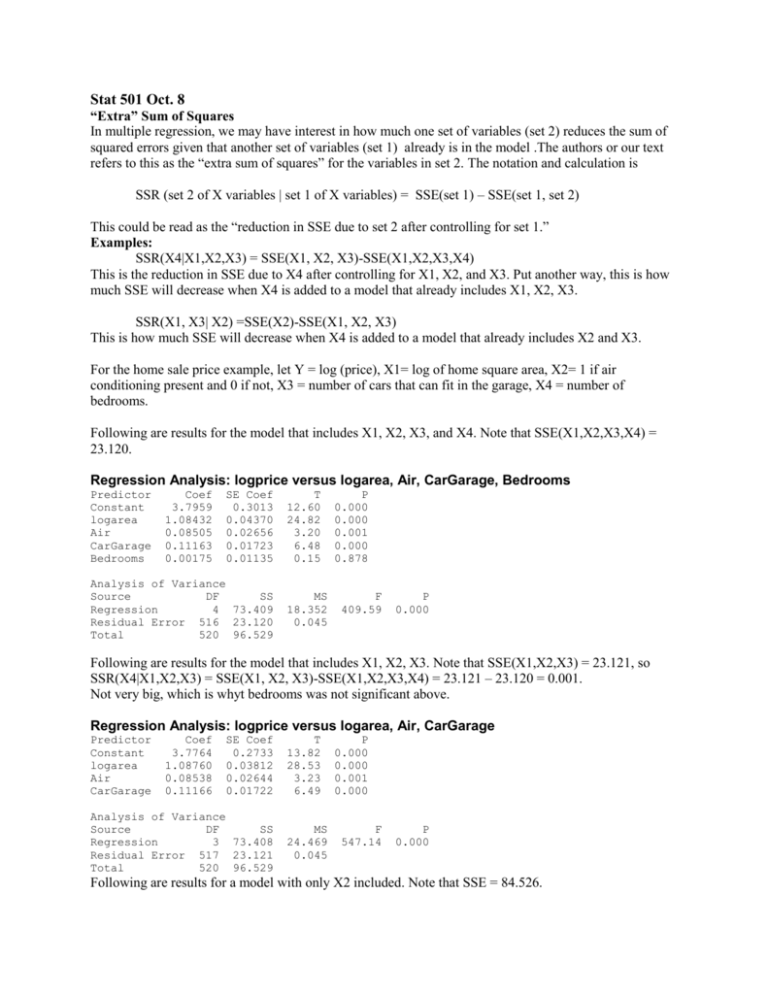
Stat 501 Oct. 8
“Extra” Sum of Squares
In multiple regression, we may have interest in how much one set of variables (set 2) reduces the sum of
squared errors given that another set of variables (set 1) already is in the model .The authors or our text
refers to this as the “extra sum of squares” for the variables in set 2. The notation and calculation is
SSR (set 2 of X variables | set 1 of X variables) = SSE(set 1) – SSE(set 1, set 2)
This could be read as the “reduction in SSE due to set 2 after controlling for set 1.”
Examples:
SSR(X4|X1,X2,X3) = SSE(X1, X2, X3)-SSE(X1,X2,X3,X4)
This is the reduction in SSE due to X4 after controlling for X1, X2, and X3. Put another way, this is how
much SSE will decrease when X4 is added to a model that already includes X1, X2, X3.
SSR(X1, X3| X2) =SSE(X2)-SSE(X1, X2, X3)
This is how much SSE will decrease when X4 is added to a model that already includes X2 and X3.
For the home sale price example, let Y = log (price), X1= log of home square area, X2= 1 if air
conditioning present and 0 if not, X3 = number of cars that can fit in the garage, X4 = number of
bedrooms.
Following are results for the model that includes X1, X2, X3, and X4. Note that SSE(X1,X2,X3,X4) =
23.120.
Regression Analysis: logprice versus logarea, Air, CarGarage, Bedrooms
Predictor
Constant
logarea
Air
CarGarage
Bedrooms
Coef
3.7959
1.08432
0.08505
0.11163
0.00175
SE Coef
0.3013
0.04370
0.02656
0.01723
0.01135
Analysis of Variance
Source
DF
SS
Regression
4 73.409
Residual Error 516 23.120
Total
520 96.529
T
12.60
24.82
3.20
6.48
0.15
MS
18.352
0.045
P
0.000
0.000
0.001
0.000
0.878
F
409.59
P
0.000
Following are results for the model that includes X1, X2, X3. Note that SSE(X1,X2,X3) = 23.121, so
SSR(X4|X1,X2,X3) = SSE(X1, X2, X3)-SSE(X1,X2,X3,X4) = 23.121 – 23.120 = 0.001.
Not very big, which is whyt bedrooms was not significant above.
Regression Analysis: logprice versus logarea, Air, CarGarage
Predictor
Constant
logarea
Air
CarGarage
Coef
3.7764
1.08760
0.08538
0.11166
SE Coef
0.2733
0.03812
0.02644
0.01722
Analysis of Variance
Source
DF
SS
Regression
3 73.408
Residual Error 517 23.121
Total
520 96.529
T
13.82
28.53
3.23
6.49
MS
24.469
0.045
P
0.000
0.000
0.001
0.000
F
547.14
P
0.000
Following are results for a model with only X2 included. Note that SSE = 84.526.
So, SSR(X1, X3| X2) =SSE(X2)-SSE(X1, X2, X3) = 84.256-23.121 = 61.135.
Adding X1 and X3 to a model that had only X2 will decrease the SSE by 72.135.
Regression Analysis: logprice versus Air
Predictor
Constant
Air
Coef
12.0965
0.40512
SE Coef
0.0430
0.04719
T
281.18
8.58
P
0.000
0.000
Analysis of Variance
Source
DF
SS
Regression
1 12.003
Residual Error 519 84.526
Total
520 96.529
MS
12.003
0.163
F
73.70
P
0.000
Testing Whether One or More Variables Can Be Dropped From the Model
A statistical test of whether a set of variables can be simultaneously eliminated as predictor variables is
based on the F-statistic
SSE (Re duced)  SSE (Full )
error
df for reduced - error df for full
F=
MSE (full )
with df = (error df for reduced – error df for full) and error df for full.
.
The precise null hypothesis is that some specified set of  coefficients is 0.
The Reduced model is the model that results if this null hypothesis is true. The Full model is the model
with all variables being considered included.
Example:
Suppose a potential model is y i   o  1 x i1   2 x i 2   3 x i 3   i . This is the “full” model.
If we wish to test
H0: 1   3  0
the reduced model is y i   o   2 x i 2   i
Basically, we’re testing to see if variables x1 and x3 are “significant” given that x2 will be in the
model. The relevant F-statistic is
SSE( x 2 )  SSE( x 1 , x 2 , x 3 )
SSR ( x 1 , x 3 | x 2 )
error df reduced  error df full
error df reduced  error df full
F

MSE ( x 1 , x 2 , x 3 )
MSE ( x 1 , x 2 , x 3 )
Tasks we’ll complete in class:
1. Consider the home price example with a full model of X1,X2,X3. Calculate an F for testing
H0: 1   3  0
2. Consider the home price example with a full model of X1,X2,X3, X4. Calculate an F for
testing H0:  4  0