Modeling Rate-dependent Hysteresis in Piezoelectric Actuators
Wei Tech Ang, Francisco Alija Garmón, Pradeep K. Khosla, and Cameron N. Riviere
The Robotics Institute, Carnegie Mellon University, Pittsburgh, PA 15213, USA
techang@cs.cmu.edu, alija@andrew.cmu.edu, pkk@ece.cmu.edu, and cam.riviere@cs.cmu.edu
Abstract – Hysteresis of a piezoelectric actuator is ratedependent. Most hysteresis models are based on elementary
rate-independent operators and are not suitable for
modeling actuator behavior across a wide frequency band.
This work proposes a rate-dependent modified PrandtlIshlinskii (PI) operator to account for the hysteresis of a
piezoelectric actuator at varying frequency. We have shown
experimentally that the relationship between the slope of the
hysteretic loading curve and the rate of control input can be
modeled by a linear function. The proposed rate-dependent
hysteresis model is implemented for open-loop control of a
piezoelectric actuator. In experiments tracking multifrequency nonstationary motion profiles, it consistently
outperforms its rate-independent counterpart by a factor of
two in maximum error and a factor of three in rms error.
I.
INTRODUCTION
A piezoelectric ceramic is an excellent choice as a
micropositioning actuator because of its high output force,
large bandwidth and fast response time. However, the
existence of nonlinear multi-path hysteresis in
piezoelectric material complicates the control of a
piezoelectric actuator in high precision applications. The
maximum hysteretic error is typically about 15% in static
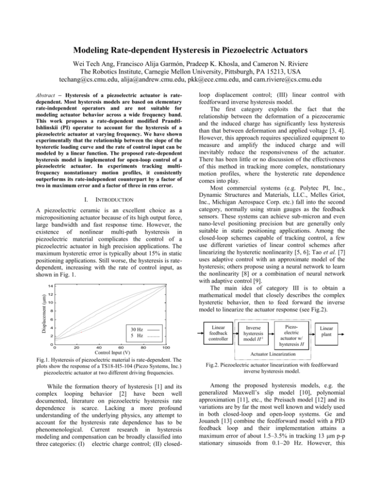
positioning applications. Still worse, the hysteresis is ratedependent, increasing with the rate of control input, as
shown in Fig. 1.
Displacement (m)
14
12
10
8
loop displacement control; (III) linear control with
feedforward inverse hysteresis model.
The first category exploits the fact that the
relationship between the deformation of a piezoceramic
and the induced charge has significantly less hysteresis
than that between deformation and applied voltage [3, 4].
However, this approach requires specialized equipment to
measure and amplify the induced charge and will
inevitably reduce the responsiveness of the actuator.
There has been little or no discussion of the effectiveness
of this method in tracking more complex, nonstationary
motion profiles, where the hysteretic rate dependence
comes into play.
Most commercial systems (e.g. Polytec PI, Inc.,
Dynamic Structures and Materials, LLC., Melles Griot,
Inc., Michigan Aerospace Corp. etc.) fall into the second
category, normally using strain gauges as the feedback
sensors. These systems can achieve sub-micron and even
nano-level positioning precision but are generally only
suitable in static positioning applications. Among the
closed-loop schemes capable of tracking control, a few
use different varieties of linear control schemes after
linearizing the hysteretic nonlinearity [5, 6]; Tao et al. [7]
uses adaptive control with an approximate model of the
hysteresis; others propose using a neural network to learn
the nonlinearity [8] or a combination of neural network
with adaptive control [9].
The main idea of category III is to obtain a
mathematical model that closely describes the complex
hysteretic behavior, then to feed forward the inverse
model to linearize the actuator response (see Fig.2).
6
4
0
Linear
feedback
controller
30 Hz
5 Hz
2
0
20
40
60
80
100
Control Input (V)
Inverse
hysteresis
model H-1
Piezoelectric
actuator w/
hysteresis H
Linear
plant
Actuator Linearization
Fig.1. Hysteresis of piezoelectric material is rate-dependent. The
plots show the response of a TS18-H5-104 (Piezo Systems, Inc.)
piezoelectric actuator at two different driving frequencies.
Fig.2. Piezoelectric actuator linearization with feedforward
inverse hysteresis model.
While the formation theory of hysteresis [1] and its
complex looping behavior [2] have been well
documented, literature on piezoelectric hysteresis rate
dependence is scarce. Lacking a more profound
understanding of the underlying physics, any attempt to
account for the hysteresis rate dependence has to be
phenomenological. Current research in hysteresis
modeling and compensation can be broadly classified into
three categories: (I) electric charge control; (II) closed-
Among the proposed hysteresis models, e.g. the
generalized Maxwell’s slip model [10], polynomial
approximation [11], etc., the Preisach model [12] and its
variations are by far the most well known and widely used
in both closed-loop and open-loop systems. Ge and
Jouaneh [13] combine the feedforward model with a PID
feedback loop and their implementation attains a
maximum error of about 1.5–3.5% in tracking 13 m p-p
stationary sinusoids from 0.1–20 Hz. However, this
method does not work for nonstationary sinusoids because
of the intrinsic properties of the classical Preisach model.
Galinaitis [14] uses a Preisach type Kransnosel’skiiPokrovskii (KP) operator to model and control
piezoelectric actuators in open loop and reports a
maximum tracking error of 3.9% with a 0.05 Hz
stationary sinusoid. The tracking errors increase to about
6–9.4% when tracking sinusoids with reduced amplitudes.
Another important subclass of the Preisach model is
the Prandtl-Ishlinskii (PI) model. The main advantages of
this approach over the classical Preisach operator are that
it is less complex and its inverse can be computed
analytically, thus making it more attractive for real-time
applications. These PI approaches reduce maximum
hysteretic error to about 1–3% in open-loop control with
quasi-static tracking [15, 16] and to about 1% in tracking
of a nonstationary constant-rate saw-tooth profile with
closed-loop adaptive control [17].
One basic assumption of the Preisach type model is
that hysteresis is rate-independent. To date, little work has
been done to explicitly model the rate dependence of
hysteresis. Tan and Baras [18] extend the Preisach
operator to model and control magnetostrictive actuators
at > 5 Hz where hysteresis can no longer be assumed to be
rate-independent. They report a maximum error of about
7.5% when tracking a nonstationary dynamic motion
profile in closed-loop control. Smith et al. [19] report that
hysteresis of piezoelectric materials is rate-dependent
even at very low frequencies (< 1 Hz).
In this paper, we present an extension to the PI
operator to also model the rate-dependent hysteresis
characteristic of a piezoelectric actuator. We implement
the rate-dependent PI hysteresis model with open-loop
control and compare the experimental results with the
rate-independent case. A discussion on the significance of
the result and the limitations of our model is also
presented.
II. PRANDTL-ISHLINSKII (PI) HYSTERESIS MODEL
This section describes the modeling of hysteresis using
the modified PI operator proposed by Kuhnen et al. [16,
17], with a slightly different treatment to account for the
one sided characteristic of many commercial piezoelectric
actuators that are driven by non-negative control voltage.
A. Prandtl-Ishlinskii (PI) Operator
The elementary operator in the PI hysteresis model is
a rate-independent backlash or linear-play operator. It is
commonly used in the modeling of backlash between
gears with one degree of freedom. A backlash operator is
defined by
y(t) = Hr[x, y0](t)
= max{x(t) – r, min{x(t) + r, y(tT)}}
(1)
where x is the control input, y is the actuator response, r is
the control input threshold value or the magnitude of the
backlash, and T is the sampling period. The initial
consistency condition of (1) is given by
y(0) = max{x(0) – r, min{x(0) + r, y0}}
(2)
with y0  , and is usually but not necessarily initialized
to 0. Multiplying the backlash operator Hr by a weight
value wh, we have the generalized backlash operator,
y(t) = whHr[x, y0](t).
(3)
The weight wh defines the gain of the backlash operator
(wh = 1 represents a 45 slope) and may be viewed as the
gear ratio in gear mechanical play analogy (see Fig.3).
y
-r
wh
x
r
Fig.3. The rate-independent generalized backlash operator
is characterized by the threshold or backlash magnitude, r, and
the weight or backlash gain, wh.
Complex hysteretic nonlinearity can be modeled by a
linearly weighted superposition of many backlash
operators with different threshold and weight values,
y(t) = whTHr[x, y0](t).
(4)
with weight vector whT = [wh0 … whn] and Hr[x, y0](t) =
[Hr0[x, y00](t) … Hrn[x, y0n](t)]T with the threshold vector r
= [r0 … rn]T where 0 = r0 < … < rn, and the initial state
vector y0 = [y00 … y0n]T. The control input threshold
values r are usually chosen to be equal intervals.
Equation (4) is the PI hysteresis operator in its
threshold discrete form. The hysteresis model formed by
the PI operator is characterized by the initial loading curve
(see Fig. 4). It is a special branch traversed by equation
(4) when driven by a monotonically increasing control
input with its state initialized to zero (i.e. y(0) = 0). The
initial loading curve is defined by the weight values wh
and threshold values r,
i
 (r )   whj (r  r j ), ri  r < ri+1, i = 0, …, n.
(5)
j 0
The slope of the piecewise linear curve at interval i is
defined by Whi, the sum of the weights up to i,
i
d
Whi   (r )   whj .
(6)
dr
j 0
The subsequent trajectory of the PI operator beyond
the initial loading curve, with non negative control input
is shown as the dotted loop in Fig. 4. The hysteresis loop
formed by the PI operator does not return to zero with the
control input and each of the piecewise linear segments
now has a threshold width of 2r because of the backlash
operators. This behavior of the PI operator closely
resembles the hysteresis of a piezoelectric actuator.
C. Parameter Identification
y
To find the hysteresis model parameters, we first have to
measure experimentally the responses of the actuator
subjected to some control inputs. Then we set the
threshold values r and d as described in the previous
section. The weight parameters wh and ws are found by
performing a least squares fit of equation (9) to the
measured actuator response.
Initial loading
curve
Whi 
i
 whj
j 0
x
ri
D. Inverse Prandtl-Ishlinskii (PI) Operator
Fig.4. The PI hysteresis model with n = 4. The hysteresis
model is characterized by the initial loading curve. The
piecewise linear curve is defined by the equally spaced threshold
values r and the sum of the weight values wh.
The inverse of a PI operator is also of the PI type. The
proof of existence of an inverse can be found in [15]. The
inverse PI operator is given by
 1[z](t) = w’hTHr’[w’sTSd’[z], y0’](t)
(10)
B. Modified Prandtl-Ishlinskii (PI) Operator
The key idea of computing the inverse is to find the
reflection of the resultant hysteresis looping curves about
the 45 line as shown in Fig. 6.
z(t) = wsTSd[x](t).
14
12
Displacement (m)
The PI operator inherited the symmetry property of the
backlash operator about the center point of the loop
formed by the operator. The fact that most real actuator
hysteretic loops are not symmetric weakens the model
accuracy of the PI operator. To overcome this overly
restrictive property, a saturation operator is combined in
series with the hysteresis operator. A saturation operator is
a weighted linear superposition of linear-stop or one-sided
dead zone operators. A dead zone operator is a nonconvex, non-symmetrical, and memory free nonlinear
operator given by
 max{ x(t )  d ,0}, d  0
S d [ x](t )  
(7)
d 0
 x(t ),
z
8
6
4
2
0
(8)
where y is the output of the hysteresis operator, z is the
actuator response, wsT = [ws0 … wsm] is the weight vector,
Sd[x](t) = [Sd0[x](t) … Sdm[x](t)]T with the threshold vector
d = (d0 … dm)T where 0 = d0 < rn < d1 < … < dm. Equal
intervals are chosen between d1 and dm. The last interval
of the hysteresis operator, rn, is selected to be at the
midpoint of the control input range (see Fig.5).
The modified PI operator is thus
z(t) =  [x](t)
= wsTSd[whTHr[x, y0]](t).
(9)
10
0
2
4
6
8
Wsi 
d0
rn d1
j 0
x
di
Fig.5. The saturation operator with m = 2. The threshold values d
have equal intervals from d1 to dm. The slope of the piecewise
linear curve at interval i is defined by the sum of the weights up
to i. The value rn is the midpoint of the full range of the control
input.
14
The inverse model parameters can be found by
 whi
1
; w' hi 
, i = 1 … n;
w' h0 
i
i 1
wh0
( whj )(  whj )
r 'i 
 wsj
12
Cascading the inverse hysteresis model with the
actual hysteresis model gives us the identity mapping
between the control input x(t) and actuator response z(t),
z(t) =  [ 1[x]](t) = I[x](t) = x(t)
(11)
j 0
i
10
Displacement Equivalent Control Input (m)
Fig.6. The solid curve is the modified PI model of a piezoelectric
actuator. The inverse model in dotted line is the mirror image of
hysteresis model about the 45 line.
i
 whj (ri  r j ),
j 0
y ' 0i 
j 0
i
n
j 0
j i 1
 whj y0i   whj y0 j ,
i = 0 … n;
(12)
wsi
1
; w' si 
, i = 1 … m;
w' s 0 
i
i 1
ws 0
( j 0 wsj )(  j 0 wsj )
i
d 'i   wsj (d i  d j ), i = 0 … m;
j 0
(13)
III.
RATE-DEPENDENT PRANDTL-ISHLINSKII (PI)
HYSTERESIS MODEL
A. Rate-dependent Hysteresis Slope
We propose in this section an extension to the modified PI
operator to also model the rate-dependent characteristics
of the piezoelectric hysteresis.
One of the advantages of the PI hysteresis model is
that it is purely phenomenological; there are no direct
relationships between the modeling parameters and the
physics of the hysteresis. Therefore we would model the
rate-dependent hysteresis with reference only to the
experimental observations.
While the rate dependency of hysteresis is evident
from Fig.1, the sensitivity of actuator saturation to the rate
of control input is not apparent. Hence we assume that
saturation is not rate-dependent and hold the saturation
weights, ws, as well as the threshold values, r and d,
constant while attempting to construct a relationship
between hysteresis and the rate of the control input x(t ) .
We model the slope of the hysteresis curve (i.e. sum of the
hysteresis weights) at time t as the sum of the referenced
hysteresis slope and a rate-dependent function,
(14)
Whi ( x(t ))  Wˆ hi  f ( x(t )), i = 1 … n.
Equation (14) will be reduced to the referenced hysteresis
slope, Ŵhi, or to the rate-independent case if the ratedependent term is zero.
B. Rate-dependent Model Identification
The response of a piezoelectric actuator is measured
subject to sawtooth control inputs at different rate values
over the range of 01200 m/s. With an amplitude of 12.5
m p-p, this corresponds to the maximum rate of
sinusoidal control input up to about 30 Hz with the same
amplitude. We perform the modified PI parameters
identification for the measured actuator response at
different rate values. The sum of the hysteresis weights
Whi, i = 0 … n, are plotted against the control input rate as
shown in Fig. 7.
Sum of weights, Whi
1.2
Wh4
Wh3
Wh2
1
Wh1
0.8
0.6
Wh0
0.4
0.2
0
200
400
600
800
1000
1200
Control Input Rate (m/s)
Fig.7. Plot of the hysteresis slopes Whi, n = 4, vs. input rate.
We observed that the hysteresis slope of the
piezoelectric actuator varies linearly with the rate of input.
Thus the rate-dependent hysteresis slope model would be:
(15)
Whi ( x(t ))  Wˆ hi  ci x(t ), i = 0 … n
where ci is the slope of the best fit line through the Whi’s
and the referenced slope Ŵhi is the intercept of the best fit
line with the vertical Wh axis or the slope at zero input
rate. The individual rate-dependent hysteresis weight
values can be calculated by
whi ( x(t ))  Whi ( x(t ))  Wh(i1) ( x(t )), i = 1 … n;
wh0 ( x (t ))  Wh0 ( x (t ))
(16)
C. Rate-dependent Modified Prandtl-Ishlinskii Operator
The rate-dependent modified PI operator is defined by
z(t) =  [x, x ](t)
= wsTSd[wh( x )THr[x, y0]](t).
(17)
The inverse rate-dependent modified PI operator is also of
the PI type:
 1[z](t) = w’h( x )THr’[w’sTSd’[z], y0’](t).
(18)
The inverse rate-dependent parameters can be found by
(12), replacing wh with the rate-dependent wh( x (t)).
IV. EXPERIMENTAL RESULTS
To model the hysteretic nonlinearity of a TS18-H5-104
(Piezo Systems, Inc.) piezoelectric actuator, we use a
modified PI model of n = 9, and m = 2, for both the rateindependent and rate-dependent case.
Fig. 8 and 9 compare the experimental results of the
rate-independent and rate-dependent PI operators tracking
a 10 Hz, 12.5m p-p stationary sinusoid and a multifrequency, nonstationary dynamic motion profile
(modulated 5, 20, and 35 Hz sinusoids with time-varying
amplitudes). The rate-independent model parameters are
identified from the measured response of the piezoelectric
actuator subjected to a 10 Hz, 12.5 m p-p stationary
sinusoidal control input.
Table 1 summarizes the
performance of the rate-independent and rate-dependent
hysteresis models in tracking experiments.
Table 1. Measured experimental errors of the rate-independent
and rate-dependent hysteresis models in tracking a 10 Hz,
12.5m p-p stationary sinusoid (Stat) and a multi-frequency,
nonstationary dynamic motion profile (Dyn).
Without
RateRatemodel
independent
dependent
Rmse
Stat
1.07
0.13
0.11
Dyn
0.84
0.40
0.11
(m)
Rmse / p-p Stat
8.6
1.0
0.9
ampl.(%)
Dyn
6.7
3.2
0.9
max error
Stat
2.07
0.33
0.34
Dyn
2.09
1.35
0.56
(m)
max error / Stat
16.6
2.6
2.7
p-p ampl.(%) Dyn
16.6
10.7
4.4
Desired
Measured
14
14
12
12
10
10
Displacement (m)
Displacement (m)
Measured
8
6
4
2
8
6
4
2
Error
Error
0
0
-2
-2
0
0.05
0.1
0.15
0
0.2
0.05
Time (s)
14
12
12
10
10
Displacement (m)
Displacement (m)
0.15
0.2
0.15
0.2
0.15
0.2
(a) Without model.
14
8
6
4
2
0
0.1
Time (s)
(a) Without model.
8
6
4
2
0
Error
-2
Error
-2
0
0.05
0.1
0.15
0.2
0
0.05
(b) Rate-independent.
14
12
12
10
10
Displacement (m)
14
8
6
4
2
0
0.1
Time (s)
Time (s)
(b) Rate-independent.
Displacement (m)
Desired
8
6
4
2
0
Error
Error
-2
-2
0
0.05
0.1
0.15
0.2
Time (s)
(c) Rate-dependent
Fig.8. Experimental open-loop tracking results of a stationary
12.5 m p-p sinusoid at 10 Hz. The rate-independent model
parameters are identified from measured response a TS18-H5104 (Piezo Systems, Inc.) piezoelectric actuator subjecting to the
same control input.
0
0.05
0.1
Time (s)
(c) Rate-dependent.
Fig.9. Experimental open-loop tracking results of a multifrequency, nonstationary dynamic motion profile. The rateindependent model parameters are identified from measured
response a TS18-H5-104 (Piezo Systems, Inc.) piezoelectric
actuator subjecting to a 10 Hz, 12.5 m p-p stationary sinusoidal
control input.
V. DISCUSSIONS
The proposed rate-dependent PI hysteresis model reports
very similar performance as the rate-independent model in
tracking a stationary sinusoid. In tracking more dynamic
motion profiles involving frequencies other than the one
on which the rate-independent model is based, the ratedependent model consistently outperforms the other by at
least a factor of two in maximum error and a factor of
three in rms error. Although the proposed model registers
a higher maximum error in the dynamic tracking case, the
rms error, a more important tracking performance
yardstick, remains almost the same.
Creep is not modeled in the proposed model because
its effect is negligible for sinusoids of > 1 Hz. If quasistatic tracking is desired, since the rate-dependent model
and its inverse are also of the PI type, the creep model
proposed by Krejci et al. [15] can be easily incorporated.
One limitation of all PI-type hysteresis models is that
it has singularity when the slope of the hysteresis loading
curve becomes zero. The inverse model near the
singularity is highly sensitive to noise and extra care has
to be taken in real-time implementation to avoid modeling
error. The singularity of the proposed rate-dependent
model occurs at around 1450 m/s or the maximum rate
of a 36 Hz, 12.5 m p-p sinusoid.
VI. CONCLUSION
We presented a rate-dependent Prandtl-Ishlinskii (PI)
hysteresis model to account for the behavior of a
piezoelectric actuator in multi-frequency tracking. The
proposed method uses a linear function to model the
relationship between the slopes of the hysteretic loading
curve and the rate of control input. Compared with a rateindependent model, our model yields significantly better
experimental results.
[6]
[7]
[8]
[9]
[10]
[11]
[12]
[13]
[14]
[15]
[16]
REFERENCES
[1]
[2]
[3]
[4]
[5]
P.Chen & S.Montgomery,“A macroscopic theory for
the existence of the hysteresis and butterfly loops in
ferroelectricity,” Ferroelect.,vol.23,pp.99-207, 1980.
M.A. Krasnosel’skii and A.V. Pokrovskii, Systems
with Hysteresis, New York: Springer-Verlag, 1989.
C. Newcomb and I. Filnn, “Improving linearity of
piezoelectric ceramic actuators”, Electronics Letters,
Vol.18, No.11, pp.442-444, May 1982.
K.Furutani, M.Urushibata, N.Mohri, “Displacement
control of piezoelectric element by feedback of
induced charge”, Nanotech., 9, pp.93-98, 1998.
B. M. Chen, T. H. Lee, C.C. Hang, Y. Guo, and S.
Weerasooriya, “An H Almost Disturbance
Decoupling Robust Controller Design for a
Piezoelectric Bimorph Actuator with Hysteresis”,
IEEE Tran. Automation and Control, Vol. 7, No. 2,
pp.160-174, Mar 1999.
[17]
[18]
[19]
C. Jan and C-L. Hwang, “Robust Control Design for
a Piezoelectric Actuator System with Dominant
Hysteresis”, Proc. 26th Annual Conf. of the IEEE
IECON 2000, Vol.3 pp.1515-1520, 2000.
G. Tao and P. V. Kokotovic, “Adaptive Control of
Plants with Unknown Hystereses”, IEEE Tran. Auto.
& Control, vol.40, no.2, pp.200-212, Feb 1995.
S-S. Ku, U. Pinsopon, S. Cetinkunt, and S. Nakjima,
“Design, Fabrication, and Real-time Neural Network
of a Three-Degrees-of-Freedon Nanopositioner”,
IEEE/ASME Trans. Mechatronics, vol. 5, no. 3,
pp.273-280, Sep. 2000.
C-L. Hwang and C. Jan, “A Reinforcement Discrete
Neuro-Adaptive Control for Unknown Piezoelectric
Actuator Systems with Dominant Hysteresis”, IEEE
Trans. Neural Net., vol.14, no.1, pp.66-78, Jan 2003.
M. Goldfarb and N. Celanovic, “Modeling
Piezoelectric Stack Actuators for Control of
Micromanipulation”,
IEEE
Control
System
Magazine, vol.17, 3, pp.69-79, June 1997.
S. Chonan, Z. Jiang, and T. Yamamoto, “Nonlinear
hysteresis compensation of piezoelectric ceramic
actuators”, J. Intell. Mater. Syst. Struct., vol.7, no.2,
pp.150-156, 1996.
I. D. Mayergoyz, Mathematical Models of
Hysteresis. New York: Springer-Verlag, 1991.
P. Ge and M. Jouaneh, “Tracking Control of a
Piezoceramic Actuator”, IEEE Trans. Control and
System Tech., Vol.4, No.3, pp.209-216, May 1996.
W. S. Galinaitis, “Two Methods for Modeling Scalar
Hysteresis and their use in Controlling Actuators
with Hysteresis”, Ph.D. Thesis, Virginia Polytechnic
Institute and State University, Blacksburg,VA, 1999.
P. Krejci and K. Kuhnen, “Inverse control of
systems with hysteresis and creep”, IEE Proc.
Control Theory Appl., vol. 148, no.3, May 2001.
K. Kuhnen and H. Janocha, “Complex hysteresis
modeling of a broad class of hysteretic
nonlinearities”, Proc. of the 8th Int. Conf. on New
Actuators, Bremen, pp. 688-691, Jun 2002.
K. Kuhnen and H. Janocha, “Adaptive Inverse
Control of Piezoelectric Actuators with Hysteresis
Operators”, Proc. Euro. Control Conf. ECC’99,
Karlsruhe, Germany, 1999.
X. Tan and J. S. Baras, “Control of Hysteresis in
Smart Actuators, Part I: Modeling, Parameter
Identification, and Inverse Control”, Technical
Research Report, CDCSS TR 2002-8, Center for
Dynamics and Control of Smart Structures, 2002.
R. C. Smith, Z. Ounaies, and R. Wieman, “A Mosel
for Rate-dependent Hysteresis in Piezoceramix
Materials Operating at Low Frequencies”, Technical
Report, NASA/CR-2001-211-62, NASA Langley
Research Center, 2001.