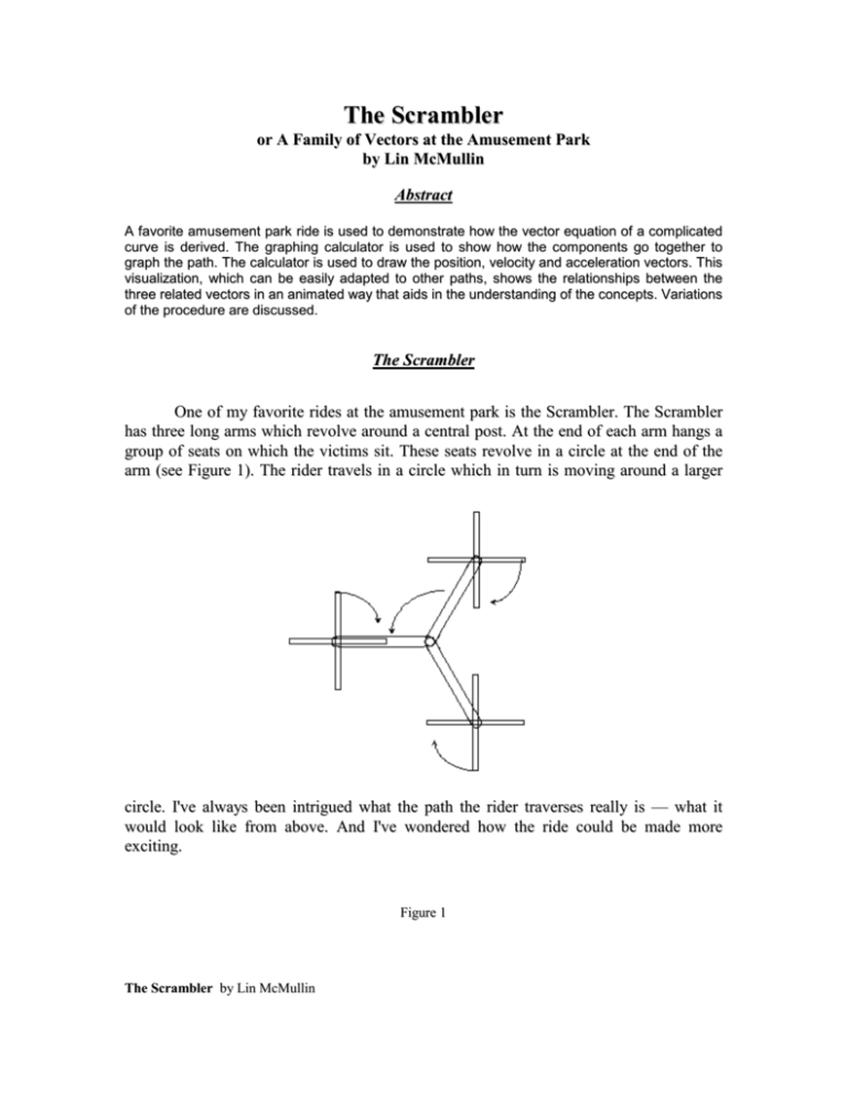
The Scrambler
or A Family of Vectors at the Amusement Park
by Lin McMullin
Abstract
A favorite amusement park ride is used to demonstrate how the vector equation of a complicated
curve is derived. The graphing calculator is used to show how the components go together to
graph the path. The calculator is used to draw the position, velocity and acceleration vectors. This
visualization, which can be easily adapted to other paths, shows the relationships between the
three related vectors in an animated way that aids in the understanding of the concepts. Variations
of the procedure are discussed.
The Scrambler
One of my favorite rides at the amusement park is the Scrambler. The Scrambler
has three long arms which revolve around a central post. At the end of each arm hangs a
group of seats on which the victims sit. These seats revolve in a circle at the end of the
arm (see Figure 1). The rider travels in a circle which in turn is moving around a larger
circle. I've always been intrigued what the path the rider traverses really is — what it
would look like from above. And I've wondered how the ride could be made more
exciting.
Figure 1
The Scrambler by Lin McMullin
The motion is fairly easy to analyze using vectors. Introduce a coordinate system

whose origin is at the center post of the Scrambler. Let OA be the vector from the origin

to the end of one of the arms, and let AB be the vector from the center of that arm to one
of the seats as shown in Figure 2. The path is represented by the various positions of the




endpoint of OB , since OB  OA  AB
Figure 2
Point A moves in a circle around the origin so it is of the form

AB  ( R1 cos(t ), R1 sin( p  t )) .
Where R1 is the radius of the longer arm and t is the angle formed with the positive xaxis. Since the Scrambler revolves at a constant rate, we may consider this angle to be our
time variable.
Point B moves around a circle with center at A so its equation is of the form

AB  ( R2 cos( p  t ), R2 sin( p  t )) . Here R2 is the length of the shorter arm.
The Parameter p
Since we will want to consider different relative speeds and directions of rotation
of the two arms the parameter p has been included in the arguments of the second vector.
The Scrambler by Lin McMullin
2

The shorter arm will rotate | p | times for each single revolution of the larger
arm.

Integral values of p will return the rider to the starting point after one full
revolution of the larger arm; non-integral values will not. Most scramblers do
not return to the starting point in one revolution.

If p > 0 both arms will revolve in the same direction (counterclockwise); if p < 0 the arms will
rotate in different directions with the shorter arms moving clockwise. Scramblers usually
rotate in different directions.
The Path
The path a rider travels is then the sum of these two vectors:
 
OA  AB  ( R1 cos(t ), R1 sin(t ))  ( R2 cos( p  t ), R2 sin( p  t )) , or

OB  ( R1 cos(t )  R2 cos( p  t ), R1 sin(t )  R2 sin( p  t ))
This equation may be easily graphed with a graphing calculator in parametric mode. Keep
R1 and R2
constant and start with p = - 2. The path is shown in Figure 3
Figure 3: The motion starts on the right at the point
(0, R1 + R2 ) and moves down and to the left.
Seeing the Component Vectors
By using the programming and drawing features of the graphing calculator one can see
the path and how the components go together to make the path. Enter the components


OA and AB separately as the first and second functions in parametric mode. Then enter
the following program in a graphing calculator (without the line numbers):
The Scrambler by Lin McMullin
3
1.
2.
3.
4.
5.
6.
7.
For n, tmin, tmax, tstep
Line 0, 0, xt1(n), yt1(n)
Line xt1(n) ,yt1(n), xt1(n) + xt2(n), yt1(n) + yt2(n)
Line 0, 0, xt1(n), yt1(n), 0
Line xt1(n) , yt1(n), xt1(n) + xt2(n), yt1(n) + yt2(n), 0
PtOn xt1(n) + xt2(n), yt1(n) + yt2(n)
EndFor
Comment on the program:
Some adjustments may be necessary depending on the model of the calculator.
Line 1: Tying the For Loop variable (n) to the window variable is a convenient way of
controlling the program.
Line 2: Draws the first vector.
Line 3: Draws the second vector attached to the end of the first vector.
Lines 4 and 5: Turn the two vectors off for clarity (some graphing calculator do not have
this capability. If so, these two lines may be omitted).
The Scrambler by Lin McMullin
4
Line 6: Turns the point on the curve on.
Figure 4: The partially drawn path showing the two
component vectors. (The origin is in the center). Note
that the points are at equally spaced time intervals
Investigating the Path
As indicated above the value of p affects the number and kind of loops on the
path. Several other paths are shown below. If p was entered in the parametric equation,
the value of p may be easily changed by storing a new value to p from the Home Screen.
Figure 5: p = -3
Figure 6: p = -4
There are (1 - p) loops when the circles revolve in different directions.
Next we look at a typical non-integral value for p. Now, after one revolution of
the large arm, the path does not end at the starting point.
The Scrambler by Lin McMullin
5
Figure 7: (left) p = - 1.8, 1 revolution and (right)
10 revolutions
Using positive values of p give very types of paths.
Figure 8: p = + 2 Figure 9; p = + 3
The Most Exciting Ride — Velocity
I suppose "the most exciting ride" depends on the rider. From the graphs above it
would appear that negative values of p give more and sharper turns and that the larger | p |
gives more turns. Referring again to Figure 4, the points are spaced at equally spaced time
intervals. The nearness of a point to the adjacent points is an indication of the speed.
Perhaps a more objective way to study the ride is to consider the velocity. To
visualize the velocity it is possible to draw the velocity vectors at any point on the curve.
This is done by using the graphing calculator's LINE operation to draw a segment whose
length and direction correspond to the velocity vector’s coordinates. Put the tail of each
vector (the first coordinates in LINE) at the corresponding point on the curve.
Differentiate the position vector to obtain the velocity vector

v  (( R1 sin(t )  R2  p  sin( p  t )), ( R1 cos(t )  R2  p  cos( p  t )))
Then write a short program to graph the lines and the path. For example enter the

path OB as xt1(t) and yt1(t) and selected (turned on) and the velocity components as
xt2(t) and yt2(t) and deselected (turned off) . Run a program with these key lines:
For n, tmin, tmax, tstep
Line xt1(n), yt1(n), xt1(n) + xt2(n), yt1(n) + yt2(n)
EndFor
The first line is a convenient way to tie the program to the parameter’s values. The
second line draws a segment from the point on the path in the direction of, and with the
length of the velocity vector at that point; that is it draws the velocity vector.
The Scrambler by Lin McMullin
6
Figure 10: Velocity Vectors At left some are drawn. At right
all drawn (p = -2)
It appears that the longest velocity vector — the fastest part of the ride — occurs
in the middle of each section. This is generally true since there must be some slowing
down to make the turns.
The same idea may be used to see the acceleration vectors. Enter the acceleration
components as xt3(t) and yt3(3). Then enter and run this program which works the same
as the last program.:
For n, tmin, tmax, tstep
Line xt1(n), yt1(n), xt1(n) + xt3(n), yt1(n) + yt3(n)
EndFor
The acceleration vectors may be large and not fit well on the screen; some resizing
of the window may be required. As you may suspect the acceleration is largest at the ends
of the loops when the direction of the velocity is changing the most; it is least when the
speed is most. The velocity and acceleration may be compared by graphing the lengths of
the velocity and acceleration vectors together as functions of time:
Figure 11: Upper graph is the length of the
acceleration vectors vs. time. Lower graph is the
speed vs. time. 0  t  2 and 0  y  60 . p =
-2
Conclusions and Extensions
The exploration above shows a method for visualizing the velocity and
acceleration vectors of a vector equation. The general procedure is to use the LINE
operation of a graphing calculator to draw the velocity or acceleration vectors at various
The Scrambler by Lin McMullin
7
points of the curve. The graphs may be produced with a simple program on any graphing
calculator with a LINE operation.



Enter the position equation in the parametric editor as xt1(t) and yt1(t). Leave
this on (selected) if you want the path drawn.
Enter the velocity equations in the parametric editor as xt2(t) and yt2(t) and
turn them off.
Enter the acceleration equations in the parametric editor as xt3(t) and yt3(t)
and turn them off.
With simple variations the entries above may be used to demonstrate

The position vectors: To draw the vectors from the origin to each point on the path
use
Line 0, 0, xt1(n), yt1(n).


The velocity the vectors: To attach the velocity vectors to the corresponding points
on the path, first draw the path and then draw the velocity vectors with
Line xt1(n), yt1(n), xt1(n) + xt2(n), yt1(n) + yt2(n).
The acceleration vectors: To attach the acceleration vectors to the corresponding
points on the path, first draw the path and then draw the acceleration vectors with
Line xt1(n), yt1(n), xt1(n) + xt3(n), yt1(n) + yt3(n)

Position and velocity vectors: Attach the velocity vectors to the ends of the position
vectors to demonstrate how the velocity vector “pulls” the position vector to its next
position by using a program with these lines
Line 0, 0, xt1(n), yt1(n)
Line xt1(n), yt1(n), xt1(n) + xt2(n), yt1(n) + yt2(n)

Velocity and Acceleration vectors: Attach the acceleration vectors to the ends of
the velocity vectors to demonstrate how the acceleration vector “pulls” the velocity
vector to its next position by using a program with
Line xt1(n), yt1(n), xt1(n) + xt2(n), yt1(n) + yt2(n)
Line xt1(n) + xt2(n), yt1(n) + yt2(n), xt1(n) + xt2(n) + xt3(n), yt1(n) + yt2(n) +
yt3(n)

Translations: To demonstrate the translation of a figure enter the equation of the
figure as xt1(t) and yt1(t) and the translating vector (two constants) as xt2(t) and
yt2(t). Then use a program with
The Scrambler by Lin McMullin
8
Line 0, 0, xt1(n), yt1(n)
Line xt1(n), yt1(n), xt1(n) + xt2(n), yt1(n) + yt2(n).
and the
Interchange the parametric equations (enter the translating vector as xt1(t) and yt1(t)
equation of the figure as xt2(t) and yt2(t)). Then run the same program.
Teaching Suggestion

Usually watching the graph being drawn is more helpful than seeing the final
graph.

Simple curves such as line, circle or parabolas work as well as complicated ones.

Circles and ellipses show nicely that the acceleration vectors always points to the
center of these curves. How long are they?

If you are studying projectile motion, Look at the horizontal and vertical
components of velocity separately by making first yt2(t) = 0 and then xt2(t) = 0.

Cycloids of various types make interesting graphs.

In picking examples be sure to check the graph window values beforehand to find
ones that work well.
Reference
These curves are called Trochoids, Roulettes, Epicycloids and Hypocycloids. (These are overlapping
categories.) For more information see Curves and their Properties by Robert C. Yates, NCTM, Reston VA,
1952, p. 233 - 236 (Trochoids), p. 175 - 185 (Roulettes) and p. 80 - 85 Epicycloids and Hypocycloids)
The Scrambler by Lin McMullin
9