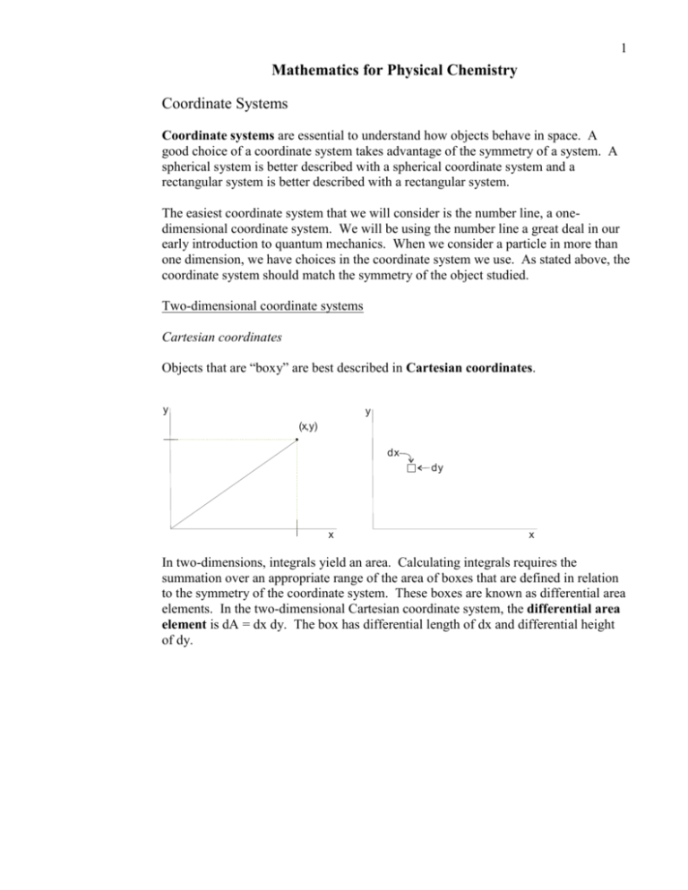
1
Mathematics for Physical Chemistry
Coordinate Systems
Coordinate systems are essential to understand how objects behave in space. A
good choice of a coordinate system takes advantage of the symmetry of a system. A
spherical system is better described with a spherical coordinate system and a
rectangular system is better described with a rectangular system.
The easiest coordinate system that we will consider is the number line, a onedimensional coordinate system. We will be using the number line a great deal in our
early introduction to quantum mechanics. When we consider a particle in more than
one dimension, we have choices in the coordinate system we use. As stated above, the
coordinate system should match the symmetry of the object studied.
Two-dimensional coordinate systems
Cartesian coordinates
Objects that are “boxy” are best described in Cartesian coordinates.
y
y
(x,y)
dx
dy
x
x
In two-dimensions, integrals yield an area. Calculating integrals requires the
summation over an appropriate range of the area of boxes that are defined in relation
to the symmetry of the coordinate system. These boxes are known as differential area
elements. In the two-dimensional Cartesian coordinate system, the differential area
element is dA = dx dy. The box has differential length of dx and differential height
of dy.
2
Polar coordinates
Objects that are approximately circular are best described with polar coordinates. The
differential area element is r dr d, that is, a box with length dr and height is r d.
y
y
(r,)
r d
r
dr
d

x
x
Transformation Equations
y
x
x  r cos 
  tan 1
y  r sin 
r  x 2  y2
Sometimes one want to describe an object in one coordinate system with another
coordinate system. The equations that are used to make the conversion are referred to
as transformation equations. Below are the transformation equations between the
Cartesian coordinate system and the polar coordinate system.
3
Three-dimensional coordinate systems
Cartesian coordinates
z
(x,y,z)
x
y
A three-dimensional integral yields a volume. Thus the calculation involves adding
3-d boxes known as differential volume elements. In the three-dimensional
Cartesian coordinate system, the differential volume element is dV = dx dy dz. The
box has differential length of dx, differential height of dy and differential depth, dz.
Differential volume element
dV = dx dy dz
z
dy
(x,y,z)
dx
dz x
y
4
Spherical polar coordinates
While Cartesian coordinates are relatively simple to use for some applications, when an
object has spherical symmetry, like an atom, stubbornly insisting on using Cartesian
coordinates to do calculations becomes very messy. Using spherical polar coordinates
for an atom is much better choice for a coordinate system because calculations become
much simpler. In the spherical polar coordinate system, r, the radial coordinate is the
distance from the origin, the polar coordinate, , is the angle from a “preferred” direction
(label as the “z” coordinate in the diagram) and the line connecting the origin with the
point. The choice of the “preferred” is usually obvious (as in the direction of the
internuclear axis connecting atoms in a diatomic molecule) or arbitrary (as in a hydrogen
atom). The azimuthal coordinate, , is the angle between the projection of line
connecting the origin and the point on the “x-y” plane (the plane perpendicular to the
“preferred” direction) and a line defining  = 0 (usually considered to the “x” axis).
z
 coordinate is like latitude
Range of  is from 0 to 
(R,,)

 coordinate is like longitude
Range of  is from 0 to 2
R
R sin 
y

x
The differential volume element is dV  r 2 sin  dr d d .
r d
z
dr


x
d
d
y
5
The transformation equations between the spherical polar coordinate system and the
Cartesian coordinate system are
x  r sin  cos 
y  r sin  sin 
z  r cos 
Cylindrical coordinates
When considering diatomic molecules (among other possible systems like molecular
spectroscopy in applied electric or magnetic fields), using the spherical polar
coordinates is awkward. It becomes more convenient to think of the molecule with
basic cylindrical symmetry rather than a spherical symmetry. Thus cylindrical
coordinates can be used.  is the radial coordinate,  is the azimuthal coordinate and
z is simply known as the height.
z
(,,z)

y

x
Transformation Equations
x   cos 
y   sin 
Differential volume element
dV   d d dz
zz
6
Complex Numbers
Introduction and Motivation
Recall the following:
Solution to x 2  1  0 is x  1
What is solution to x 2  1  0
x 2  1  0  x 2  1  x  1
What is 1 ?
Define i  1 .
Note: i  i  1  1  1
i 2  1
What is solution to x 2  2x  5  0 ?
Find solution from quadratic equation.
x
b  b2  4ac 2  4  20
1

 1
16  1  2i
2a
2
2
Complex number may have two parts
z  a  bi
a – real part
b – imaginary part
7
Representations of complex numbers
Argand plane
While real numbers can be plotted on a number line, complex numbers must be
plotted on a plane (called the Argand plane).
Rectangular coordinates
(a+ bi)
b
a
Polar coordinates
A complex number can also be represented in polar coordinates.
(a+ bi)
r sin 
r

r cos 
a  bi  r cos   i r sin   r  cos   isin 
a  r cos 
b  r sin 
r  a 2  b2 - modulus
b
  tan 1   - phase angle
a
Without proof, the following identity will be asserted
Euler’s identity: e i  cos   i sin 
Therefore a complex number in rectangular coordinate can always be expressed in
polar coordinates and vice versa.
a  bi  r ei
8
Operations with complex numbers
We will need to add complex numbers together as well as multiplying them.
Addition of complex numbers
Adding complex numbers in the rectangular representation is simple. The sum is
simply the sum of the real part and the sum of the imaginary part.
(a + bi) + (c + di) = [(a + c) + (b + d)i]
Addition in the polar representation is enormously difficult. In practice, numbers in
the polar representation are converted to the rectangular representation, added, and
then reconverted to polar representation.
Multiplication of complex numbers
Multiplying numbers in the rectangular representation is performed with the same
technique as multiplying binomials; with the FOIL method (keeping in mind that i ∙ i
= –1).
(a + bi) × (c + di) = (a × c) + (a × di) + (bi × c) + (bi × di)
= ac + adi +bci + bdi2
= ac – bd + (ad + bc)i
Multiplying numbers in the polar representation is easier. The moduli are multiplied
together and the phase angles are added.
u = (r1, 1) v = (r2, 2) u ∙ v = (r1 ∙ r2, 1 + 2)
9
Double and Triple Integrals
Double Integrals
Recall integration of a single variable.
x 
y
x 2  x1
n
x2
n
 f (x) dx  lim f (x i ) x
n 
x1
i 0
xi  x1  i(x)
Integration is a
summation of rectangle
x
x2
x1
x
areas to yield an area under a curve.
What if the bottom border of an area is not the x-axis?
f(x)
y
Area between the
curves
A
x2
 f (x)  g(x) dx
x1
Rather than use
g(x) rectangles with uniform
x, we could vary x.
x1
y
x
x2
x
f(x)
Note two limiting
processes are needed.
One for the xcoordinate and one for
the y-coordinate.
y
g(x)
x1
x
x2
x
A
x 2 f (x)
 
x1 g(x)
 same as above
dy dx 
x2
y
x1
f (x)
g(x)
dx 
x2
 f (
x1
10
Examples:
1 4
1
3x 2
3x
dx
dy

0 2
0 2
1
 3  4 2 3  2 2 
dy   

 dy  18 dy  18y |10  18
2
2

0 
0

1
4
2
Note that for multiple integrals, there exist a defined order to the integrations.
Integrations are done “from the inside, out”. In the above example, dx is “inside” dy;
therefore, the “x” integration is done first, then the “y” integration. Note that the
limits of 2 to 4 are “inside” the limits of 0 to 1; therefore, the 2 to 4 limits are used in
the “x” integration and the 0 to 1 limits are used in the “y” integration.
2 4
2
  dx dy   x
0 2y
dy    4  2y dy  4y  y 2
0
2
2 y
2

1
2
4
2y
x dx dy  
1
y

 3
 8  4  (0  0)  4
0
x2
2
y2
y
2
 y4 y 
y5 y 2
dy      dy  
2 2
10 4
1 
2
1
32 4  1 1  31 3 62 15 47
      


10 4  10 4  10 4 20 20 20

  r sin  dr d   sin  d
3
0 0
2
0
0
3
3
 r dr   cos 
0

0
r4
4
3
0
81
81 81
 81 
   cos     cos 0     0      1    1  
2

4
4 2
4

Triple Integrals
Evaluation of triple integrals yields a volume instead of an area.
Parallelpipeds (boxes) are summed rather than rectangles.
Examples:
2 2x y  x
 
1 x
0
2  2
 r
0 0 0
2 2x
2
 y2

dy dx     y  x  dy dx     xy 
2

1 x
1 x
1 
2
2 
2
  x2
2x 


x2
  
 x  2x     x  x   dx   dx
 2
  2
2
 
1 
1


x3 2 8 1 7

 
1 
6
6 6 6
2 2x
dz dy dx    z
yx
0
2
5
sin  dr d d   r dr
5
0

2
0
0
2x
x
dx
 sin  d  d 
r 2
32
128

2
2 2 
0  cos  0  0 
6
3
3
Note that in the integral above, the integrand can be separated into three independent
functions and that the bounds of integration have no functional dependencies.
Therefore, the triple integral is the same as the product of three single integrals.
We’ll find this circumstance a great deal in quantum chemistry.

6
11
Vector Differential Operators
Introduction
In quantum chemistry, many of the quantities we will consider are vector quantities.
(Review your knowledge of vectors, including dot products and cross products from
physics.) That is, the quantities will have a magnitude and a direction. The electric
force between charges is a vector quantity as is the electric field emanating from a
collection of charges. The dipole moment of a molecule is a vector quantity. The
flow of a liquid is a vector quantity. Other quantities are simpler in that they only
have a magnitude. Such quantities are called scalar quantities. Examples of scalar
quantities are charge, electric potential, temperature.
We often want to know how scalar quantities and vector quantities change. Recall
from calculus that a change in a quantity is a derivative. Thus to find the changes of
quantities all we need to is take a derivative. However, because vector quantities
have direction and scalar quantities can change independently in each of the three
spatial dimensions; we have to be careful about what we mean by a derivative. We
will examine three kinds of vector derivatives, the gradient, the divergence and the
curl.
All the vector derivatives involve a vector quantity called the del operator. The
symbol for the del operator is an upside-down delta, .
Del operator in Cartesian coordinates

 ˆ  ˆ  ˆ
i
j k
x
y z
Del operator in spherical polar coordinates


1 
1 
eˆ r 
eˆ  
eˆ 
r
r 
r sin  
12
Gradient

The gradient operator operates on a scalar quantity to find how the scalar quantity
changes in three orthogonal directions. The del operator is applied to the scalar
quantity to find its gradient. Thus the change of a scalar quantity is a vector quantity.
Since the gradient is a vector quantity, it has a direction.
**The direction where the gradient points is the direction of maximum change of the
scalar quantity.**
Example: Within a 2 meter cubic box, the temperature has been measured and found
to be a function of x, y and z. T  x, y, z    x 2  y 2 z  273 K . The thermal energy
will flow from the box in the opposite direction of the maximal change of the
temperature. Thus q  T
a) Calculate the gradient of the temperature function.
 

 
T   ˆi  ˆj  kˆ   x 2  y 2 z  273
y
z 
 x

  x 2  y 2 z  273
x
 2x ˆi  2yz ˆj  y 2 kˆ
ˆi 
  x 2  y 2 z  273 
y
ˆj 
  x 2  y 2 z  273 
z
kˆ
b) Calculate the value of the gradient at the point x = 1 m, y = 1 m and z = 2 m.


2
T  2x ˆi  2yz ˆj  y 2 kˆ  T  2 1 iˆ  2 1 2  ˆj  1 kˆ  2 iˆ  4 ˆj  kˆ K m
c) Find the angle between the direction of thermal energy flow at the point x =
1 m, y = 1 m and z = 2 m and the x = 1 plane of the box.
The x = 1 plane is perpendicular to the unit vector in the x direction. Recall the
definition of the dot product, A  B  A B cos  . Let A  ˆi and B  2 ˆi  4 ˆj  kˆ


A  B  A B cos   ˆi  2 ˆi  4 ˆj  kˆ  ˆi 2 ˆi  4 ˆj  kˆ cos 

  2  0  0  1  2    4   1
 cos  
2
2

1
2 2
cos    2  21 cos 
2
 2 
   cos 1 
  2.02 rad  115.88
21
 21 
13
Divergence
F
The divergence operator is one of two operators used to find the derivative of a
vector-valued function, that is, a function that has a value and direction everywhere in
space. The flux of a vector-valued function to or away from enclosed volume is
found by taking the divergence. The divergence is found by taking the dot product of
the del and a vector-valued function to yield a scalar quantity. (In coordinates other
than Cartesian coordinates, the calculation is more sophisticated.) Consider the flow
of gas through a section of pipe. The divergence of the flow tells about how the flow
is changing. Consider three different possibilities.
1) If the divergence of the flow is zero, the gas flowing into the section equals
the gas flowing out of the section.
2) If the divergence is positive then the flow of gas into the pipe is less than the
flow of gas out of the pipe. Thus overall, the pressure of the gas is increasing.
The section of pipe contains a source of gas.
3) If the divergence is negative then the flow of gas into the pipe is more than the
flow of gas out of the pipe. Thus overall, the pressure of the gas is decreasing.
The section of pipe contains a sink of gas.
Example: The flow of a polymer solution through a flexible Tygon tube is profiled as
the following vector-valued function,
F  x, y, z   214 ˆi   2y  0.098y3  ˆj   2z  0.098z3  kˆ  mol in .
The coordinate system origin is at the start of the tube and the middle. Is the fluid
expanding or compressing? When will the divergence be zero?
The flux of a vector-valued function to or away from a point is found by taking the
divergence.


 
  F   ˆi  ˆj  kˆ    214 ˆi   2y  0.098y3  ˆj   2z  0.098z 3  kˆ 
y
z 
 x
  214    2y  0.098y


x
y
3
    2z  0.098z 
3
z
 0   2  0.294y 2    2  0.294z 2   4  0.294y 2  0.294z 2
14
We don’t know if the fluid is expanding or compressing because we don’t the radius
of the tubing, that is, we don’t know y and z. Let us find the radius of the tubing
when the divergence equals zero.
  F  4  0.294y2  0.294z 2  0  4  0.294r 2  r 
4
 3.69
0.294
Thus when the tube is smaller than 3.69 in, the divergence is positive and the tube
will expand to 3.69 in. If the tube is larger than 3.69 in, the divergence is negative
and the tube will contract to 3.69 in.
Curl
F
The curl operator is used to find the derivative of a vector-valued function
perpendicular to its flow. **A nonzero curl means that the flow is rotating.** The
curl of a vector-valued function is found by taking the cross product of the del
operator and the vector-valued function.
Example: Is the flow in the above problem rotating?


 
  F   ˆi  ˆj  kˆ    214 ˆi   2y  0.098y3  ˆj   2z  0.098z 3  kˆ 
y z 
 x
3
3
  214  ˆ ˆ   2y  0.098y  ˆ ˆ   2z  0.098z  ˆ ˆ

ii 
i j 
ik
x
x
x
3
3
  214  ˆ ˆ   2y  0.098y  ˆ ˆ   2z  0.098z  ˆ ˆ

j i 
j j 
j k
y
y
y
 
 
 
 
 
 
  214  ˆ ˆ   2y  0.098y

ki 
z
z
 
3


 
kˆ  ˆj 
  2z  0.098z3 
z
 
  F   0  0    0  kˆ   0  ˆj
 

  0   ˆj   0   ˆi    2  0.294z   0 
  0   kˆ   2  0.294y 2   0    0  ˆi
2
0
Thus, the flow is not rotating.
 kˆ  kˆ 
15
Laplacian
   2
The divergence of a gradient of a scalar function is the Laplacian of the scalar function.
**The Laplacian is a three-dimensional second derivative of a multi-variable scalar
function.** The Laplacian is a scalar function itself. In quantum mechanics, the Laplacian is
used to express the kinetic energy of a microscopic particle.
Laplacian in Cartesian coordinates
2 
2
2
2


x 2 y2 z 2
Laplacian in spherical polar coordinates
2 
1
 2 
1
 
 
1
2
r

sin






r 2 sin  r  r  r 2 sin   
  r 2 sin 2  2
Table of vector derivative operators.
Cartesian coordinates.
Gradient
 
 ˆ  ˆ  ˆ
i
j
k
x
y
z
Divergence
V 
Vx Vy Vz


x
y
z
Curl
 V V   V V   V V 
 V   y  z  ˆi   z  x  ˆj   x  y  kˆ
y   x
z   y
x 
 z
Laplacian
   2 
 2  2  2


x 2 y2 z 2
16
Spherical coordinates
Gradient
 
Divergence
V 
 1 
1 


r r  r sin  
1  2
1 
1 
r Vr  
V
 sin  V  

2
r r
r sin  
r sin  
Curl
 V 



1  


  

  r sin V    rV  eˆ r  r  Vr   r sin V  eˆ   r sin    r V   Vr  eˆ  
r sin   

r
  
 r

 

2
Laplacian
   2 
1   2 
r
r 2 r  r
Differential Equations
1
 
 
1
 2


sin


 2


  r 2 sin 2  2
 r sin   
17
Introduction
What are differential equations? Consider an analogy with algebraic equations.
Algebraic equation: 2x  6  0  x  3
x  3 is the solution to the equation
Differential equation:
dy
y0
dx
What y = f(x) solves the equation?
Try y = ex
dy
 y  e x
dx
 ex  ex  0
ex is not a solution to the differential equation.
Try y = e-x
y  e x  e x  e x  0
e-x is a solution to the differential equation.
Types of differential equations
Partial – diff. eq. with partial derivatives (solutions are multi-variable functions)
 2  2  2


 4
x 2 y2 z 2
Ordinary – diff. eq. with ordinary derivatives (solutions are single variable
functions)
2
dy
m2
2 d y
1  x  dx 2  2x dx  l  l  1 y  1  x 2 y  0
Linear – diff. eq. with the form ay  by  cy  dy 
 f x
All terms in the equation have derivatives raised to the first or zeroth power.
Nonlinear – diff. eq. that is not linear
One or more terms in the equations have derivatives raised to the second or higher power.
Order of a differential equation – highest derivative within equation
18
Examples in the classification of differential equations
y  cos x
y  k 2 y  0
y  yy  4  0
first order, linear
second order, linear
third order, nonlinear
y  7  y   8y  0
3
second order, nonlinear
Separable Equations
Separable differential equations can be rewritten as integrals.
Consider the following differential equation.
dy
 y  f (x)
 dy  f (x) dx

dx
y   f (x) dx
 dy   f (x) dx

Thus, a simple first-order differential equation is the same thing as an indefinite
integral.
The technique of separable equations is to separate all that depends on each variable
to different sides of the equation and integrate.
Consider the following example involving the first-order kinetics of nuclear decay.
Example: Radioactive decay is proportional to the number of nuclei. If N = N0 at
time t =0, find the number of atoms at time t.
dN
 N
dt
 - decay constant
First separate variables N and t.
dN
  dt
N
Now integrate
N
t
dN
N N  0  dt 
0
ln N
 ln N  ln N 0  ln
or
N
N0
 t
N
 t
N0
N  N 0 e t
t
0
19
Example: The first-order kinetics of radioactive decay is well described with a firstorder differential equation that can be solved with separation of variables
technique. For 14C,  = 1.750  10-4 yr-1. If an animal bone is assumed to
have 1.0 mol of 14C at death and the bone is measured to have 0.13 mol
presently, how old is the bone?
ln
N
 t
N0

t
1 N
1
0.13 mol
ln

ln
 12000 yr
4
1
 N 0 1.750 10 yr
1.0 mol
Linear First-order Equations
The general form for a linear first-order equation is y  P  x  y  Q  x 
The solution for the a general linear first-order equation is
y  e I  Q(x)e I dx  c e  I where I   P(x)dx and c is a arbitrary constant
that depends on the specific “boundary values” of the problem.
20
1
, find y
x
First manipulate equation as to find P and Q.
1
2
1
x 2 y  2xy 
 y  y  3
x
x
x
Example: If x 2 y  2xy 
Px  
2
x
Qx 
1
x3
I   P  x  dx  
2
dx  2 ln x
x
e I  x 2
e I  e2ln x  eln x  x 2
1
y  x 2  3 x 2 dx  c x 2  x 2  x 5dx  c x 2
x
1 4
1
 x2
x  c x2  2  c x2
4
4x
2
Check solution
1
x 3
y   2x 3   2c x 
 2c x
4
2
 x 3

1
 1
 1
x 2 y  2xy 

x2 
 2c x   2x  2  c x 2  
x
 4x
 x
 2

 x 1
  1
 1
 2c x 3   
 2c x 3  

 x
 2
  2x
1
1
1

 2c x 3  2c x 3 

2x 2x
x
1
1
0
x
x
Example: Find the solution for the differential equation: y  y  ex
I   dx  x  y  e  x  e x e x dx  ce  x
 y  e  x  e 2x dx  ce  x
1
1 
y  e  x  e 2x   ce  x  e x  ce  x
2
2 
Check solution
1
y  e x  ce  x 
2
y  y  e x
1
1
 1
 1
  e x  ce  x    e x  ce  x   e x  e x  e x
2
2
 2
 2
21
Homogeneous first-order equations
General linear homogeneous first-order equation: y  P(x)y  0
Note: Q(x) = 0
 P(x)dx
Solution: y  c e 
If P(x) is a constant then y  c1e P x
All first-order homogeneous diff. eq. will have an exponential solution.
Technique using auxiliary equation
d
dy
 y
Let D 
so that Dy 
dx
dx
Then y  P(x)y  0 
Dy  Py  0   D  P  y  0 - auxiliary equation
The “roots” of the auxiliary equation are the values of the exponents.
D  P  0  D  P  y  c1e Px
Homogeneous second-order equations
General linear second-order equation: A(x)y  B(x)y  C(x)y  D(x)
For a homogeneous second-order equation, D(x) = 0.
If A(x), B(x) and C(x) are constants, then the second-order equation can be rewritten
as a product of first-order equations. The solution of each first-order differential
equation is an exponential function; thus, the solution of the second-order equation is
a sum of exponential functions.
d
dy
d2 y
For the following, let D 
so that Dy 
and D2 y  2 .
dx
dx
dx
Example: Solve y  5y  4y  0
y  5y  4y  0 

D

 D  4 D  1 y  0
 D  4 y  0 or  D  1 y  0

2
 5D  4  y  0
D2 y  5Dy  4y  0
(auxiliary equation)
dy
 4y  0  y  c1e4x
dx
dy
 y  0  y  c2e x
 D  1 y  0 
dx
The general solution is y  c1e4x  c2e x
 D  4 y  0

22
Thus the solution of differential equation depends on finding the exponents for the
exponential functions.
***These exponents can be found by finding the roots of the auxiliary equation.***
D
2
 5D  4  y  0
 a 2  5a  4  0
 a  4, 1
Worth noting is that the roots of the auxiliary equation can be complex so the solution
of the differential equation can involve complex exponential functions.
Digression: Application of Differential Equations to the Harmonic Oscillator.
Pure Harmonic Oscillator
Consider a mass connected to a spring.
-x
+x
x0
Hooke’s Law: Force of a spring is proportional to its displacement from equilibrium
F  k  x  x 0 
k – spring constant (force constant, Hooke’s Law constant)
When the coordinate system is defined conveniently to let x0 = 0, then F  k  x
For a harmonic oscillator: Force of acceleration equals the force from Hooke’s law
F  ma  m
d2x
dt 2
d2x k
 x0
dt 2 m
F  kx
m
d2x
 kx
dt 2
x = x(t)
equation for a pure harmonic oscillator
For our later convenience, let define
k
 2
m
Equation for a pure harmonic oscillator becomes
d2 x
 2 x  0
2
dt
23
Let us now apply the auxiliary equation technique to find a solution to harmonic
oscillator equation. (The solution relates the position of the mass to the time elapsed.)
d
D2 x  2 x  0 

dt
D2  2  D  i
D
D
2
 2  x  0
Thus the solution to the pure harmonic oscillator is x  c1eit  c2eit
Recall Euler’s identity e it  cos t  i sin t
Using Euler’s identity, the solution can be rearranged to x  c3 cos t  ic4 sin t
***Thus the solution for a pure harmonic oscillator is a sinusoidal wave.***
Damped Harmonic Oscillator
A frictional force on the spring can be introduced as a term that is proportional to the
velocity
Fd  d
dx
dt
d – damping constant
The differential equation from equates the spring force with the inertial force
becomes:
d2x
dx
d 2 x d dx k
m 2  kx  d


 x0
dt
dt
dt 2 m dt m
d
 2b
For convenience, let us define
m
The auxiliary equation becomes:  D 2  2bD  2  x  0
The roots of the auxiliary equation are D  b  b2  2
Consider three cases of damping
Case I: b 2  2 Overdamped oscillator
Solution: x  c1e1t  c2e2 t
- mass returns to equilibrium quickly
- no oscillation around equilibrium point
Case II: b 2  2 Critically damped oscillator
Solution: x   c1  c2 t  et
- mass returns to equilibrium in infinite time
- no oscillation around equilibrium point
24
Case III: b 2  2 Underdamped oscillator
Solution: x  et  c1eit  c 2e it 
- mass returns to equilibrium in infinite time
- oscillation occurs around equilibrium point
- amplitude of oscillations decreases over time
- oscillations have decay envelope
Underdamped harmonic oscillator with decay envelope
1
1
0.5
t
cos( 8  t) e
t
e
0
t
e
0.5
1
1
0
2
4
6
0
8
10
12
t
14
12.56
Comparison of Damped Oscillators
y  4y  4  0
Critically damped:
y  3y  4  0
Underdamped:
y  5y  4  0
Overdamped:
1.5
 2t
e
1.5
( 1 2  t)
 1  e 4t  e t
 2
0
cos 7  t e
 1.5t
 1.5 1.5
0
0.5
1
0
Linear Algebra/Matrix Algebra
1.5
2
t
2.5
3
3.5
4
4
25
Definitions
Rows, Columns and Elements
a b c


M  d e f 
g h i 


row 1
row 2
row 3
column 3
column 2
column 1
Diagonal
a



e 


i 

For a single element of the matrix, Mrow, column
For example, M11 = a, M13 = c, M21 = d, M32 = h
Transpose
Flip matrix along diagonal
I. e., row 1  column 1 row 2  column 2
a d g


b e h
c f i 


etc …
1 4 2
 1 8 3




T
M  8 7 1   M   4 7 9
3 9 3
 2 1 3




Determinant
Definition for a 2  2 matrix
a b
a b
M
 ad  bc
  det M 
c d
c d
 1 4 
Example: Find det M where M  

2 5 
det M  1 5   4  2  5  8  13
For a 3  3 matrix
a b c
e f
d f
d e
d e f a
b
c
h i
g i
g h
g h i
 aei  afh  bdi  bfg  cdh  ceg
Shortcut for 3  3 matrices only!
+ + +
- - a b c a b
d e f
g h i
d e  aei  bfg  cdh  ceg  afh  bdi
g h
26
 1 5 2 
Example: Find det W where W   7 3 4 
 2 1 5 


1 5 2 1 5
7 3 4 7 3  1 3 5    5  4  2    2  7 1   2  3  2   1 4 1   5  7  
2 1 5 2 1
 15  40  14  12  4  175  144
Matrix Operations
Addition
To add two matrices together, matrices must be same size. Elements in
the same row/column position are added together.
 7 3 2 
 9 6 11


Example: Calculate P + Q where P   4 8 1  and Q   0 3 5 
 0 2 4 
1 2 2 




 7 3 2   9 6 11  7  9 3  6 2  11  2 3 13 

 
 
 

P  Q   4 8 1    0 3 5    4  0 8  3 1  5    4 5 6 
 0 2 4   1 2 2   0  1 2  2 4  2   1 0 6 

 
 
 

Multiplication by a scalar (constant)
Multiply every element by the scalar
Example: Calculate 4P
 28 12 8 


4P   16 32 4 
 0 8 16 


Multiplication of matrices
To multiply matrices the number of columns of the first matrix must equal
the number of rows of the second matrix.
The i,j element of the product matrix is formed by taking the “dot product”
of the ith row of the first matrix with the jth column of the second matrix.
 4 2 
 1 3 
Example: If A  
 and B  
 , calculate AB
1 9 
 4 2 
27
 4 1  2  4  4  3  2  2    12 16 
AB  


 11  9  4  1 3  9  2    35 15 
Example: For A and B given in the problem above, calculate BA
1 2   3  9    1 29 
 1 4   3 1
BA  


 4  4   2 1 4  2   2  9    14 26 
**NOTE: AB  BA In other words, matrix multiplication is not
commutative.**
1 0 2
1 1 0




Example: Calculate AB – BA when A   3 1 0  and B   0 2 1 
0 5 1
 3 1 0 




11  0  0   2  3 11  0  2   2  1 1 0   0 1  2  0    7 1 0 

 

AB   3 1  1 0   0  3 3 1  1 2   0  1 3  0   1 1  0  0     3 1 1 
 0 1  5  0   1 3 0 1  5  2   1 1 0  0   5 1  1 0    3 9 5 


 
 11  1 3  0  0  1 0   1 1  0  5  1 2   1 0   0 1   4 1 2 

 

BA   0 1  2  3  1 0  0  0   2  1  1 5  0  2   2  0   11    6 3 1 
 3 1  1 3  0  0  3  0   1 1  0  5  3  2   1 0   0 1   0 1 6 


 
 7 1 0   4 1 2   3 0 2 

 
 

AB  BA   3 1 1   6 3 1    3 2 2 
 3 9 5   0 1 6   3 8 1 

 
 

Inverse of a matrix
The inverse of matrix, A-1, obey the following matrix multiplication properties
AA-1 = A-1A = 1
1 0 0 0
1 0 0 

1 0 
 0 1 0 0
1 

  0 1 0 
0 1 0 0 1 0 0 1 0

 

0 0 0 1
Finding the inverse of a matrix in general is not too difficult but it is more than we
want to consider here. The inverse for any 2  2 matrix is given below.
a 
a
1  a 22 a12 
A   11 12   A 1 


det A  a 21 a11 
 a 21 a 22 
Systems of Equations
28
Matrix algebra can be used to solve for n unknowns in n equations. Of the many
methods possible, we will briefly consider two.
Gaussian Elimination
Consider the following set of equations.
2u  v  w  1
4u  v  2
4u  2v  w  9
What are the values for u, v and w?
Let put this system of equations in matrix form.
 2 1 1  u   1 

   
 4 1 0  v    2 
 4 2 1  w   9 

   
Gaussian elimination entails using the following manipulations on a system. These
manipulations do not change the solution of u, v and w.
1) Multiply a row by a number.
2) Add two rows together.
To use the technique efficiently, we create an “expanded matrix” composed of the
coefficient matrix and the vector of constants.
 2 1 1  u   1 
 2 1 1 1

   


 4 1 0  v    2    4 1 0 2 
 4 2 1  w   9 
 4 2 1 9 

   


We will use the above operations to change the expanded matrix into an upper
triangular matrix, that is, the coefficients below the diagonal will be zero.
a b c x


0 d e y
0 0 f z 


Then u, v and w can be found be simple substitution.
To begin let us eliminate element 2,1 from the expanded matrix. We can do this by
multiplying the first row by –2 and adding it to the second row.
29
 2 1 1 1


 4 1 0 2  
 4 2 1 9 


 4 2 2

  0 1 2
 4 2 1

2
2
2 
 4 2 2 2 
 4




 4 1 0 2    4  4 1  2 0  2 2  2 
 4 2 1 9 
 4
2
1
9 



2 

4 
9 
Now let us eliminate element 3,1 by multiplying row 1 by –1 and adding to row 3.
2
2
2 
 4 2 2 2 
 4 2 2 2
 4






1
2
4 
 0 1 2 4    0 1 2 4    0
 4 2 1 9 
 4 2 1 9 
 4  4 2  2 1  2 9  2 






4 2 2 2 


  0 1 2 4 
 0 4 3 11 


Now let us eliminate element 3,2 by multiplying row 2 by 4 and adding to row 3.
2 
2
2
2 
4 2 2 2 
4 2 2
4






8
16 
 0 1 2 4    0 4 8 16    0 4
 0 4 3 11 
 0 4 3 11 
 0 4  4 3  8 11  16 






2 
4 2 2


  0 4 8 16 
 0 0 5 5 


This matrix can now be used to find our results. Let us use the matrix to recreate our
system of equations.
2 
4u  2v  2w  2
4 2 2
 4 2 2  u   2 



  

 0 4 8 16    0 4 8  v    16   4v  8w  16
 0 0 5 5 
 0 0 5  w   5 
5w  5



  

We can now use each equation in turn to find u, v and w.
5w  5  w  1
4v  8w  16   4v  8 1  16   4v  8  v  2
4u  2v  2w  2  4u  2  2  2 1  2  4u  4  u  1
This technique is often very handy and much more efficient than raw substitution
(which will work but is very tedious with algebra).
Cramer’s rule
30
Another method for solving systems of equations is Cramer’s rule. This method is
especially handy if you have a computer program that can quickly calculate the
determinants of matrices.
Each unknown is solving by taking the ratio of two determinants. The denominator
of each ratio is always the determinant of the coefficient matrix. For our example
above,
 2 1 1  u   1 

   
 4 1 0  v    2 
 4 2 1  w   9 

   
2
1 1
4 1 0   2 11  1 0  4   1 4  2    2  0  2   1 4 1  11 4   10
4 2 1
The numerator of each ratio is the coefficient matrix with a column replaced by the
constants vector. To solve for u, the first column is replaced with the constants
vector.
1
1 1
2 1 0
9 2 1
111  1 0  9   1 2  2   1 0  2   1 2 1  11 9   10  1
u

2 1 1  2 11  1 0  4   1 4  2    2  0  2   1 4 1  11 4  10
4 1 0
4 2 1
To solve for v, the second column is replaced with the constants vector.
2
1
1
4 2 0
4 9 1  2  2 1  1 0  4   1 4  9    2  0  9   1 4 1  1 2  4  20
v


2
2 1 1
 2 11  1 0  4   1 4  2    2  0  2   1 4 1  11 4  10
4 1 0
4 2 1
To solve for w, the third column is replaced with the constants vector.
2
1
1
4 1 2
4 2 9
 2 1 9   1 2  4   1 4  2    2  2  2   1 4 9   11 4   10  1
w

2 1 1
 2 11  1 0  4   1 4  2    2  0  2   1 4 1  11 4  10
4 1 0
4 2 1
Eigenvalues and Eigenvectors
1 3
For the 2  2 matrix, 
 , the eigenvalue/eigenvector problem is stated as
 2 2
31
1 3  x 
x

    
 2 2  y
 y
x
What are values of  (eigenvalues) and the vectors   (eigenvectors) that make the
 y
above equation true?
Restatement of the problem: Multiplying a square matrix by an arbitrary vector
yields another vector. When the resultant vector is a multiple of the arbitrary vector,
we say that particular vector is an eigenvector. The scalar multiple is called the
eigenvalue.
The eigenvalue/eigenvector problem can be restated as
1 3  x 
x

      0 
 2 2  y
 y
1 3  x 
1 0  x  1 3  x    0   x 

    
   
   
 
 2 2  y
0 1  y  2 2  y  0   y
 1 3    0    x   1  
3  x
 

     
    0
2    y
 2 2   0     y   2
This last equation is called the characteristic equation of the matrix.
To solve for the eigenvalues and eigenvectors of a matrix.
1. Find the eigenvalues by calculating the determinant of the matrix in the
characteristic equation.
3  x
1  

   0
2  y
 2
1 
3

 1    2     3  2   0
2
2
 2  3   2  6   2  3  4  0
2. Set the determinant equal to zero and solve for the roots of the equation. The
roots of the equation are the eigenvalues.
 2  3  4  0     1   4 
   1, 4
3. Each dimension of the square matrix yields an eigenvalue. A 2  2 has two
eigenvalues. A 3  3 matrix has three eigenvalues, etc… Each eigenvalue
corresponds to an eigenvector. The eigenvalues are used to find the eigenvectors.
32
To find the eigenvectors, a relationship must be found be x and y of the unknown
eigenvector.
a) This relationship is found by plugging an eigenvalue into the characteristic
equation of the matrix.
3  x
1   1
3  x
1  
0


   0   2
2   1   y 
2  y
 2

 2 3  x 
2
 
     0  2x  3y  0  y   x
3
 2 3  y 
b) Thus the eigenvector in its most general form is
 x 
v 2 
  x 
 3 
All of the following eigenvectors are valid eigenvectors for the eigenvalue, -1.
 3 

 1 
3

6
     4 


v 2   

    2   4   1 
  
 3
 2 
The preferred eigenvector is called a normalized eigenvector.
Normalization will be considered shortly.
c) Find the other eigenvector associated with the other eigenvalue.
3  x
1   4 
3  x
1  
0


    0   2
2   4    y 
2   y
 2

 3 3   x 
 
     0   3x  3y  0  y  x
 2 2   y 
x
This eigenvector for the eigenvalue, 4, in its most general form is v   
x
 1 2 1 


Example: The eigenvectors for the matrix Z   2 3 0  are
 1 0 3


1
0
5
 
 
 
v1   2  , v 2   1 and v3   2  . Find the eigenvalues corresponding to each
2
 1 
1
 
 
 
eigenvector.
33
 1 2 1  1   11  2  2   11   4 
1
  

  
 
Z   2 3 0  2    2 1  3  2   0 1    8   4  2 
 1 0 3  1   11  0  2   3 1   4 
1

  
 
  
Thus the eigenvalue is 1  4
 1 2 1  0   1 0   2  1  1 2    0 
0
  

  
 
Z   2 3 0  1   2  0   3  1  0  2     3   3  1 
 1 0 3  2   1 0   0  1  3  2    6 
2

  
 
  
Thus the eigenvalue is 2  3
 1 2 1  5   1 5   2  2   1 1   10 
 5
 

  

 
Z   2 3 0  2    2  5   3  2   0  1    4   2  2 
 1 0 3  1   1 5   0  2   3  1   2 
1

  

 
 
Thus the eigenvalue is 3  2
Normalization of eigenvectors
The square of a normalized eigenvector is one. In other words, the dot product
between a normalized eigenvector and itself is one.
n n 1
Eigenvectors are normalized by multiplying them by an appropriate constant.
Nv Nv  1  N 2 v v  1  N 
1
vv
34
 x 
x
Example: Normalize the following eigenvectors: v    , v   2  .
  x 
x
 3 
x
v v   x x     2x 2
x
1
1
1


2
vv
2x
2x
 1 
1 x  2 

Therefore the normalized eigenvector is n  Nv 
 
2x  x   1 


 2
N
 x 
2 
13

v v   x  x  2   x2 N 
3    x  9

 3 
1
1
3


vv
13 2
13x
x
9
 3 
 x  

3 
   13 
Therefore the normalized eigenvector is n  Nv 
2
13x   x   2 
 3  

 13 