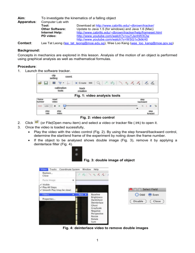
Aim:
Apparatus:
Contact:
To investigate the kinematics of a falling object
Computer Lab with
Tool:
Other Software:
Internet Help:
PD video:
Download at http://www.cabrillo.edu/~dbrown/tracker/
Update to Java 1.5 (for windows) and Java 1.6 (Mac)
http://www.cabrillo.edu/~dbrown/tracker/help/frameset.html
http://www.youtube.com/watch?v=cuYJsnhWXOw
http://www.youtube.com/watch?v=WSG1x3klkH0
Lee Tat Leong (lee_tat_leong@moe.edu.sg), Wee Loo Kang (wee_loo_kang@moe.gov.sg)
Background:
Concepts in mechanics are explored in this lesson. Analysis of the motion of an object is performed
using graphical analysis as well as mathematical formulas.
Procedure:
1. Launch the software tracker.
Fig. 1: video analysis tools
Fig. 2: video control
2.
3.
Click
(or File|Open menu item) and select a video or tracker file (.trk) to open it.
Once the video is loaded sucessfully,
 Play the video with the video control (Fig. 2). By using the step forward/backward control,
determine the start/end frame of the experiment by noting down the frame number.
 If the object to be analysed shows double image (Fig. 3), remove it by applying a
deinterlace filter (Fig. 4).
Fig. 3: double image of object
Fig. 4: deinterlace video to remove double images
1

Select the display of the clip settings by clicking clip settings
. set the Start and End
frames to define the range you wish to analyze. In this training video, set start frame to be
“4” and the end frame as “17”. Click on OK to proceed.
Fig. 5: clip setting
Fig. 6: Changes to video control (compare to Fig. 2)
4.
To calibrate the scale on the video, click the calibration tool
and select calibration
stick. For this video, the 1.000 m metre rule is on the video, move it to capture the length as in
the video.
Fig. 7: calibration tools
5.
Set the reference frame origin and angle. Click the Axes
to show the coordinate axes.
Drag the origin and/or x-axis to set the reference frame origin and angle. A common choice for
the origin is the initial position of an object of interest. (Rotation of axes can be achieved via
the tick mark on the horizontal axis, notice the status above the video
.)
2
6.
Click Create
and choose a track type from the menu of choices. Most moving
objects are tracked using a Point Mass.
Fig. 8: create track for tracking object


Mark its position on every frame by holding down the shift key and clicking the mouse
(crosshair cursor) as the video automatically steps through the video clip (Fig. 9). Track
the ball until end of frame. (Note: don't skip frames--if you do, velocities and accelerations
cannot be determined.)
The Plot View displays graphs of track data (Fig. 9). To plot multiple graphs, click the
Plots button and select the desired (3) plots number. Click the x- or y-axis label to change
the variable plotted on that axis. In this video, choose y versus t, vy versus t & ay versus t.
+ mouse click
Fig. 9: tracking of the object and its kinematics graphs
7.
Right-click on a plot (y versus t) and choose analyse… in the popup menu. Select the various
options as shown in the figure.
3
Fig. 10: graphical analysis

8.
9.
Select points you want to perform a curve fit. For this exercise,
o select “Parabola” Fit Equation of the form y = a*t^2 + b*t + c,
o select “Autofit”,
o take a look at the parameters and values
Repeat Steps 7 for plot (vy versus t) and use the “Linear” Fit Equation y = a*t + b
Right click on the plot of vy versus t and select Analyze-Area and select by click and drag the 2
grey vertical boundaries (the boundary may be hard to see, move the mouse cursor around the
plot area until you see the cursor turn to ↔, click and drag to move the boundary) to select the
area to measure for the duration of start of motion to the start of 1st bound of the ball. Calculate
the area under a velocity-time graph.
Drag the
grey lines
Fig. 11: Graphical analysis using area
4
10. Define potential energy, and total energy, via “data builder” (access through “Track Control”).
Fig. 12: defining constants and functions
5