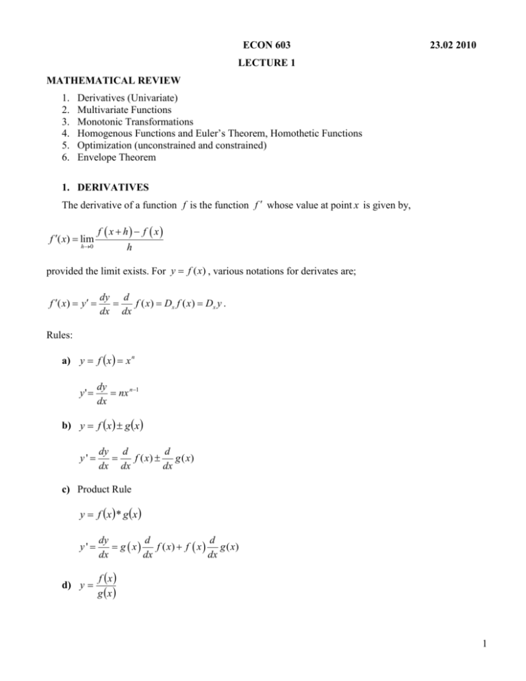
ECON 603
23.02 2010
LECTURE 1
MATHEMATICAL REVIEW
1.
2.
3.
4.
5.
6.
Derivatives (Univariate)
Multivariate Functions
Monotonic Transformations
Homogenous Functions and Euler’s Theorem, Homothetic Functions
Optimization (unconstrained and constrained)
Envelope Theorem
1. DERIVATIVES
The derivative of a function f is the function f  whose value at point x is given by,
f ( x)  lim
h 0
f  x  h  f  x
h
provided the limit exists. For y  f ( x) , various notations for derivates are;
f ( x)  y 
dy d

f ( x)  Dx f ( x )  Dx y .
dx dx
Rules:
a) y  f x   x n
y' 
dy
 nx n 1
dx
b) y  f x  g x
y'
dy d
d

f ( x)  g ( x)
dx dx
dx
c) Product Rule
y  f x  * g x 
y' 
d) y 
dy
d
d
 g  x
f ( x)  f  x  g ( x)
dx
dx
dx
f x 
g x 
1
dy
y'

dx
g  x
d
d
f ( x)  f  x  g ( x)
dx
dx
2
 g  x  
e) Chain Rule
y  f  z  where z  g x
y  f g x
y'
dy dy dz
 *
dx dz dx
Examples:
y  z 3 where z  8x 2
By substitution;
 
y  8x 2
3
and take
dy
dx


y'  83 * x 6  83 * 6 * x 5  3072 x 5
with chain rule;
 
dy dy dz

*
 3z 2 * 16 x  3 8 x 2
dx dz dx
2
*16 x  3072 x 5
f) Derivative of ln x and ex (transcendental functions)
y  log a x means a y  x
y  log a g ( x) 
Ex: 52  25  log 5 25  2
dy
g ( x)

dx g ( x).ln a
The natural logarithm ln ;
u  ln a implies eu  a with base being the irrational number e  2.7182818459....
Then;
y  ln f ( x) 
dy
1
d
f ( x)

*
f ( x) 
dx f ( x) dx
f ( x)
2
Examples:
y  ln x  y 
1
x
y  ln 3x  y 
1
1
*3 
3x
x
y  ln 6 x3  y ' 
1 df ( x)
1
1
 3 *18 x 2  x
f ( x) dx
6x
3
The exponential function e x ;
y  e x  y' 
dy
 ex
dx
d f  x
d
e
 e f  x
f  x
dx
dx
y  e 6 x  y'  e 6 x *18x 2
3
3
2. MULTIVARIATE FUNCTIONS
Given the multivariate function y  f ( x1 , x2 , x3 ,.........xn )
a) Partial derivative: The effect of a change in an independent variable xi , on the dependent variable y
holding other variables constant.
(For example: the statement that ‘the marginal utility of some good xi is positive’ means that if xi is
increased by some amount xi , holding the other goods ( xi ’s) constant, the resulting change in total
utility will be positive. This is nothing but taking the partial derivative of marginal utility with respect to
xi , holding the other variables constant.)
y  f ( x1 , x2 )
From now on we will use the notation
f1 
f
; (holding x2 constant) and
x1
f2 
f
;
x 2
(holding x1 constant)
3
Example:
f ( x, y)  ax 2  bxy  cy 2
f1 
f
 2ax  by
x
and f 2 
f
 bx  2cy
y
Second Derivatives:
f 12
 f 
 
x
    b and
y
f 21
 f 
 
y
   b
x
by Young’s Theorem f12  f 21
Example: (Silberberg and Suen p40)
If the consumer’s utility function is given by U ( x1 , x2 )  x1 log x2 the marginal utility derived from
consuming good x2 is;
U2 
U x1
 ,
x2 x2
U 22 
U 2
x
  12 , implying diminishing marginal utility.
x2
x2
(the partial derivative w.r.t. x2 , holding x1 constant), and
b) Total Derivative: change in the dependent variable due to an infinitesimally small change in one of the
independent variable when all the independent variables are allowed to change.
Consider the function:
y  f ( x1 , x2 ) , (so there are three variables, one dependent and two independent)
f ( x1 , x2 )  y0 , where y0 is a pre-assigned constant value, represents the level curves of the function. (level
curves; two dimensional graphs of three dimensional functions). This equation can be solved for one of
the unknowns in terms of the other as,
x2  x2 ( x1 ) and hence f functions becomes, f ( x1 , x2 ( x1 ))  y0 .
4
Then since we defined x2 explicitly as a function of x1 , the slope of any level curve,
dx2
makes sence.
dx
Then, total derivative of y  f ( x1 , x2 ) is defined as;
df dx1 df dx2 dy0


0
dx1 dx1 dx2 dx1 dx1
 f1  f 2
dx2
0
dx1
Then the slope of the level curve is,

dx2
f
  1 , assuming f 2  0
dx1
f2
For y  f ( x, z ) ,
dy f ( x, z ) dx f ( x, z ) dz f ( x, z ) f ( x, z ) dz




dx
x dx
z dx
x
z dx
Then the ‘Total Differential’, the total change in y is defined as
f ( x, z )
f ( x, z )
dx 
dz
x
z
 f1 dx  f 2 dz
dy 
Example: y  x 2 z 3 where z  2 x compute the total derivative of y with respect to x.
dy y y dz


===> total derivative
dx x z dx
 2 xz 3  3 x 2 z 2
dz
 2 xz 3  6 x 2 z 2
dx
Example: (Silberberg and Suen p50)
If the level curve is the production function y  F ( L, K ) , the slope is,
f
dK
  L , showing that the slope measures the willingness of firms to substitute labor for capital,
dL
fK
because it measures the benefits of additional labor f L , to the output loss due to using less capital f K .
Also, if the marginal products of each factor input are positive, then the isoquants will have a negative
slope, so, downward sloping.
5
Similarly, the slope of an indifference curve expresses that the willingness of a consumer to make
exchanges is based on the ratio of perceived gains and losses from such an exchange.
d 2 x2
To show the convexity of the indifference curve we need to show
 0 as well. Following the
dx12
necessary steps explained in the textbook (Silberberg and Suen, p52) we derive that;
d 2 x2
1
 ( f 22 f11  2 f1 f 2 f12  f12 f 22 ) 3
2
dx1
f2
So convexity of the indifference curve does not imply or implied by “diminishing marginal utility, (that is
f11  0 and f 22  0 ). The cross effect f12 must be considered as well.
Example: Monopolist Output
Q  1000  10 P
Monopolist ==> only provider ==> as quantity changes price changes too. So in a monopolist market
price is a function of the quantity.
P  100 
1
Q
10
TR  P * Q , a function of two variables.
Computing MR necessitates taking the total derivative of TR
MR 
dTR TR TR dP
 1


*
 P  Q   and substitute P
dQ
Q
P dQ
 10 
 100 
1
1
1
Q  Q  100  Q
10
10
5
c) Application of Chain Rule to Multivariate Functions
y  f x1 , x2  where x1  x1 t  & x2  x2 t  ====> x1, x2 are functions of t.
As t changes, x1 and x2 change and hence y changes. So y is a function of t.
y  f x1 t , x2 t   yt   y'  ?
dx
dx
dy y dx1 y dx2


 f1 1  f 2 2
dt x1 dt x2 dt
dt
dt
6
Example:
y  log  x1  x 2 
x1  x1 t   t
x 2  x 2 t   t 2
dx
dx
dy
 f1 1  f 2 2
dt
dt
dt
1
1

1
2t
x1  x 2
x1  x 2
y' 

1
1  2t 
x1  x 2
Substitute x1 and x2 ====>
1
1  2t 
t  t2
Example:
The function y  F ( x1 ,...xn ) is an explicit function of the independent variables.
The function G( x1 , x2 ,..., xn , y)  0 defines the dependent variable y as an implicit function of the
independent variables x1 ,..., xn .
f  x, y   0  implicit function
f ( x, y )  x 2  y 2  1  0  y '  ?
dx 2 dy 2 d 1


0
dx
dx
dx
 dy 2 dy 2 dy 
dy

2x  2 y
 0  0.........

dx
dx
dy
dx


dy
x

dx
y
Example: 4 xy3  x 2 y  x 3  5 x  6  0  y ' 
dy
?
dx
dy
dy
 2 xy  x 2
 3x 2  5  0
dx
dx
dy
 12 xy 2  x 2
 5  4 y 3  2 y  3x 2
dx
3
dy 5  4 y  2 y  3x 2

dx
12 xy 2  x 2
 4 y 3  12 xy 2


7
3. MONOTONIC TRANSFORMATIONS
Utility function U  U ( x1 , x2 ) , shows an ordinal ranking of the preferences.
The following utility function V conveys the same information as U and preserves the same ordinal
ranking;
V ( x1 , x2 )  F (U )  F (U ( x1 , x2 )) ,
where F (U )  0 .
Then,

U and V move in the same direction

V is a monotonically increasing function of U .
(and if F (U )  0 V is a monotonically decreasing function of U )

Here F relabels the level curves of U giving them new numbers
Terminology: Monotonically increasing  Monotonic
Example: U ( x1 , x2 ) is a utility function
V  logU ( x1 , x2 ) is a monotonic transformation of U .
V  eU ( x1 , x2 ) is another monotonic transformation of U .
First Partial Derivatives of Monotonic Functions
How can the partial derivatives of V ( x1 , x2 )  F (U )  F (U ( x1 , x2 )) be interpreted in terms of partial
derivatives of U ?
V1  F (U )U1
V2  F (U )U 2
Then the slope of the level curve;
dx2
V
F U1
U
 1 
 1
dx1
V2
F U 2
U2
is unaffected by this relabeling of the indifference curve. (So the MRS is preserved under monotonic
transformations.
8
However, diminishing marginal utility is not preserved under monotonic transformations, since
‘diminishing marginal utility’ has no meaning in the context of ordinal utility.
V11  F U11  F U12
V22  F U 22  F U 22
V12  V21 by Young’s Theorem.
Obviously U11  0 and U 22  0 , U11 and V11 do not necessarily have the same sign, (WHY?)
4. HOMOGENOUS FUNCTIONS AND EULER’S THEOREM
A function f ( x1 , x2 ,..., xn ) is said to be homogenous of degree “r” if
f (tx1 , tx2 ,..., txn )  t r f ( x1 , x2 ,..., xn )
Example:
Y  L K 1  f L, K 
f tL, tK   tL tK 

1
homogenous of degree 1
 t  L t 1 K 1  t
 tL K 1  tf L, K 
Theorem 1: (p59 Silberberg and Suen)
If f ( x1 , x2 ,..., xn ) is homogenous of degree r, then, the first partial f1 , f 2 ,..., f n are homogenous of degree
r-1.
Euler’s Theorem
Suppose f ( x1 , x2 ,..., xn ) is homogenous of degree r, then,
f
f
f
f
x1 
x2 
x3  ... 
xn  rf  x1 , x2 , x3 ,..., xn 
x1
x2
x3
xn
Example Page 65 Q1 a)
f x1 , x2   x1 x22 show that the function is homogenous and verify Euler’s Theorem.

f tx1 , tx2   tx1 tx2   t 3 x1 x22  t 3 f x1 , x22
2

 homogenous of degree 3.
9
Euler’s Theorem
f
f
x1 
x 2  3 f  x1 , x 2 
x1
x 2
f
 x 22 ,
x1
f
 2 x1 x 2
x 2
then  x 22 x1  2 x1 x 22  3 x1 x 22  3 f  x1 x 2 
Homothetic Functions
A homothetic function is a monotonic transformation of a function that is homogenous of degree 1.
(Homothetic functions are functions whose MRTS (slope of the level curve) is homogeneous of degree
zero. Therefore along any ray through the origin, level curves have the same slope, so that theyare radial
blow-ups of each other.
5. OPTIMIZATION
Unconstrained Optimization
For f ( x1 , x2 ) , conditions for
Relative Max
Relative Min
f1 , f 2  0
f1 , f 2  0
f11 , f 22  0
f11 , f 22  0
f11 f 22  f122  0
f11 f 22  f122  0
Comments
1.
f11 f 22  f122  0 ==> if f11 and f 22 both have the same sign ==> infection point.
==>if f11 and f 22 have different sign ==> saddle point.
2.
f11 f 22  f122  0 ==>test is inconclusive
10
Constrained Optimization
Problem:
maximize
f ( x, y )
(the objective function)
subject to
g ( x, y )  k
(the constraint)
Solution is done through the Lagrange function;
L  f ( x, y )   (k  g ( x, y ))
The choice variables ( x*, y*) and the Lagrange multiplier  * are derived through solving the first order
conditions (f.o.c.). Substituting solution in the objective function yields the ‘indirect objective function’
f *( x*, y*) . It shows the maximum values of the objective function f at point ( x*, y*) .
Meaning of Lagrange Multiplier (λ)
λ approximates the effect of a small change in constraint, on the optimum of objective function.
Case (Silberberg p 167): Suppose that the problem is output maximization subject to a resource (say
labor), constrained at level L . If the constrained resource increases by an additional increment, L , then
output will increase by Q   *L . So it appears that  * is the marginal value of that resource. In a
competitive economy, firms would be willing to pay  * for each increment in the resource. Then,  * is the
shadow price of that resource.
For a cost minimization problem  * measures the change in the total cost if input changes. So it is
marginal cost.
If the problem is utility maximization subject to the budget constraint, then λ becomes the marginal utility
of income.
11
6. ENVELOPE THEOREM
The Envelope Theorem is about creating a new function out of a set of functions by choosing the optimum
value of every function in the set.
f * ( y )  min f ( x, y )
x
f ( x1 , y )
f ( x2 , y)
f ( x2 , y)
f *( y )
y
The theorem says that the slope of the envelope at any point is the same as the slope of every single
function it touches.
Then how does an indirect objective function f * vary (as compared to objective function f ) when an
exogenous variable changes?
The theorem enables us to measure the effect of a change in an exogenous variable on the optimal value of
the objective function, by taking derivative of the Lagrange function and evaluating the derivative at the
value of the optimal solution.
This is a very useful tool. Below envelope theorem is proved for unconstrained and constrained
optimization.
-Unconstrained Model
maximize y  f ( x1 , x2 ; ) , two variables and a parameter  .
Solution gives each choice variable xi  xi ( ) , in terms of the parameter.
Substituting in the objective function we get
y* ( )  f  x1* ( ), x2* ( ),    indirect object function
Then to see the effect of a change in  on the maximum value of the objective function, we take the
derivative of the indirect objective function’s derivative w.r.t. .
12
y* ( ) 
x*
x*
f x1* f x2* f


 f1 1  f 2 2  f
x1  x2  


But since f1  f 2  0 by the f.o.c. given above,
y* ( )  f is the rate of change of f as  varies (holding x1 , x2 constant). (1)
In other words the change in the indirect objective function when one parameter of the problem is
changed, is equal to the change in the objective function. But what does the change in the indirect
objective function mean??? It is the change in the objective function when x is chosen optimally. So the
change in the objective function when we change  and we adjust x optimally, is the same as the change
when we do not adjust x optimally.
-Constrained Model
maximize
f ( x1 , x2 ,..., xn ;  )
subject to
g ( x1 , x2 ,..., xn ;  )  y
L  f   ( g  y)
f.o.c.
L x  fx1  g xi  f i  g i  0
L  f   g   0
L  g  0
 xi  xi* ( )
  *i ( )
Then, substitute this into the object function and get y * , the indirect objective function;
y* ( )  f  x1* ( ),..., xn* ( );  
then, how does y * ( ) change as α changes?
==>
y * f x1*
f xn* f

 ....................

 x1 
xn  
(2)
xi*
i fi   f
Pay attention that f i  0
Take the derivative of the constraint with respect to α
13
==>  g i
i
xi*
 g  0

(3)
(2) + (3) (multiply (3) by λ)
x*
x*
x*
dy *
  fi i  f    gi i   g    fi   gi  i  f   g  L
d



i
i
(4)
So the Envelope Theorem tells us that
-
for the unconstrained model y* is the same as f  , (1)
-
for the constrained model y*  L . (4)
14