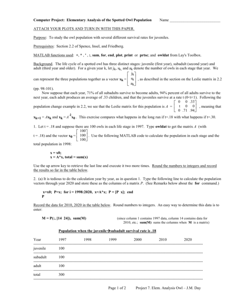
Computer Project: Elementary Analysis of the Spotted Owl Population
Name __________________________
ATTACH YOUR PLOTS AND TURN IN WITH THIS PAPER.
Purpose: To study the owl population with several different survival rates for juveniles.
Prerequisites: Section 2.2 of Spence, Insel, and Friedberg.
MATLAB functions used: +, * , ' , :, sum, for, end, plot, print or prtsc; and owldat from Lay's Toolbox.
Background. The life cycle of a spotted owl has three distinct stages: juvenile (first year), subadult (second year) and
adult (third year and older). For a given year k, let j k, sk, and ak denote the number of owls in each stage that year. We
 jk
can represent the three populations together as a vector xk =  sk , as described in the section on the Leslie matrix in 2.2
a
 k
(pp. 98-101).
Now suppose that each year, 71% of all subadults survive to become adults, 94% percent of all adults survive to the
next year, each adult produces an average of .33 children, and that the juveniles survive at a rate t (0<t<1). Following the
 0 0 .33
population change example in 2.2, we see that the Leslie matrix for this population is A =  t 0 0 , meaning that
 0 .71 .94
k
xk+1 = Axk and xk = A x0 . This exercise compares what happens in the long run if t=.18 with what happens if t=.30.
1. Let t = .18 and suppose there are 100 owls in each life stage in 1997. Type owldat to get the matrix A (with
 100
t = .18) and the vector x0 =  100 . Use the following MATLAB code to calculate the population in each stage and the
 100
total population in 1998:
x = x0;
x = A*x, total = sum(x)
Use the up arrow key to retrieve the last line and execute it two more times. Round the numbers to integers and record
the results so far in the table below.
2. (a) It is tedious to do the calculation year by year, as in question 1. Type the following line to calculate the population
vectors through year 2020 and store these as the columns of a matrix P. (See Remarks below about the for command.)
x=x0; P=x; for i = 1998:2020, x=A*x; P = [P x]; end
P
Record the data for 2010, 2020 in the table below. Round numbers to integers. An easy way to determine this data is to
enter:
M = P(:, [14 24]), sum(M)
(since column 1 contains 1997 data, column 14 contains data for
2010, etc.; sum(M) sums the columns when M is a matrix)
Population when the juvenilesubadult survival rate is .18
Year
1997
1998
1999
2000
2010
2020
--------------------------------------------------------------------------------------------------------------------------------------juvenile
100
--------------------------------------------------------------------------------------------------------------------------------------subadult
100
--------------------------------------------------------------------------------------------------------------------------------------adult
100
--------------------------------------------------------------------------------------------------------------------------------------total
300
--------------------------------------------------------------------------------------------------------------------------------------Page 1 of 2
Project 7. Elem. Analysis Owl – J.M. Day
(b) Type the following line to plot curves for the data in each of the three age groups. Because yr is a row vector
the same shape as each row of P, the command plot(yr, P) will plot row one of P against yr, then row 2 against
yr, etc. Using plot this way causes the three graphs to appear in different colors and line types on the same axes.
yr = 1997:2020; plot(yr, P)
(c) Label your curves ("Adult," "Subadult," "Juvenile"). Print your graph. (See Remarks below.)
3. Now let t = .30 and repeat the instructions of question 2 to verify that the population of owls will not die out if the
survival rate of juveniles to subadults is .30 instead of .18 . To begin, type A(2,1) = .30 and then use  to retrieve the
line with the for loop, so you do not have to type it again.
Plot the new data, label curves, print graph, and record data in the table below. Round numbers to integers.
Population when juvenilesubadult survival rate is .30
Year
1997
1998
1999
2000
2010
2020
-------------------------------------------------------------------------------------------------------------------------------------juvenile
100
-------------------------------------------------------------------------------------------------------------------------------------subadult
100
-------------------------------------------------------------------------------------------------------------------------------------adult
100
-------------------------------------------------------------------------------------------------------------------------------------total
300
-------------------------------------------------------------------------------------------------------------------------------------4. Repeat the calculations and plotting in question 3 for these additional values of t: .20, .24, .26, .28.
You do not have to record data or print graphs for these, but just list all the values of t for which your
calculations suggest that the population of owls seems to survive: _____________________________________
Remarks:
The command for i = 1998:2020 ... end is a loop; it causes MATLAB to perform the intermediate commands for
each value of i, so 23 times. At each step, the command x = A*x calculates the new x and then the command
P = [P x] adjoins that new x to the columns already in P. Notice the final P has 24 columns (why?).
To learn more about for and sum, see the MATLAB boxes in the Study Guide, or type help for and help sum.
In MATLAB 4 or 5, you can print the current graphics screen by typing the command print. Or you can click on a
graphics screen to display it, and then choose Print in the pulldown File Menu on that screen.
In MATLAB 3.5, type prtsc to print the graphics screen. You may need to execute the DOS command graphics
before prtsc will work. For example, on the Command screen, type
!graphics
prtsc
Alternatively, if your keyboard has a key labeled Prtscr, pressing that may cause the graphics screen to be printed
If necessary, consult your instructor or lab assistant, or just copy the graph by hand.
Page 2 of 2
Project 7. Elem. Analysis Owl – J.M. Day