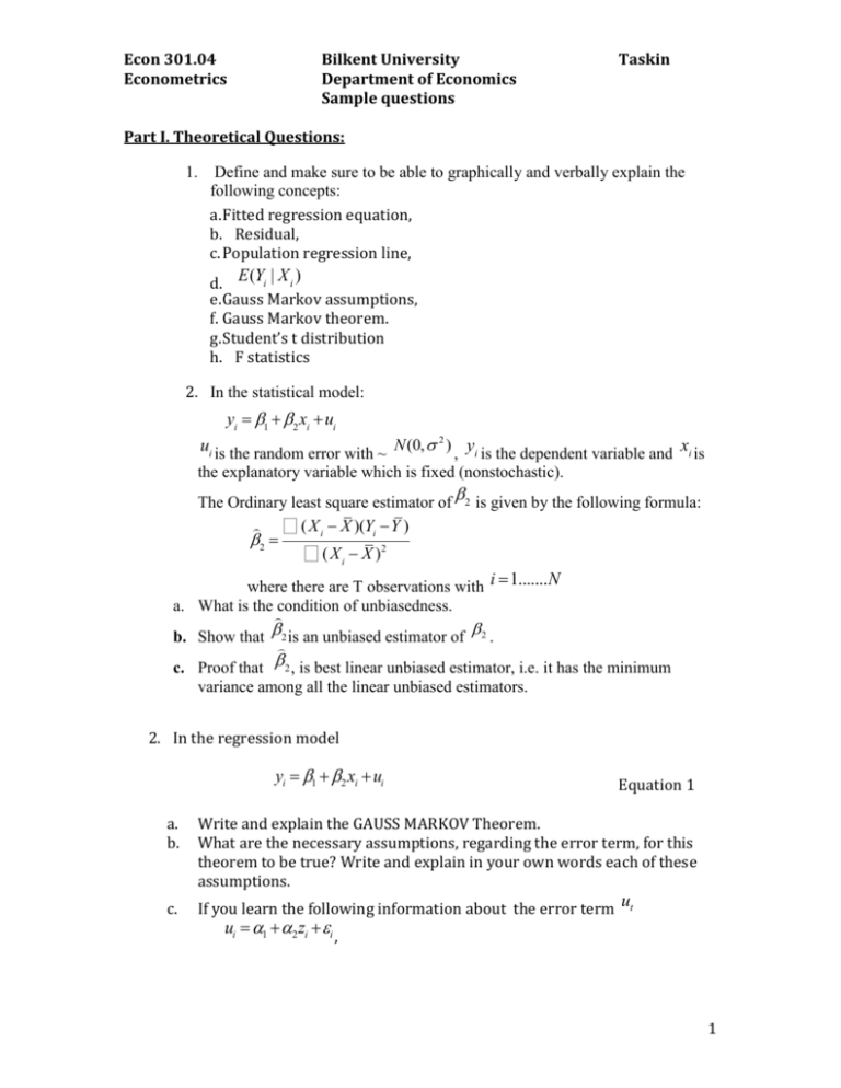
Econ 301.04
Econometrics
Bilkent University
Department of Economics
Sample questions
Taskin
Part I. Theoretical Questions:
1.
Define and make sure to be able to graphically and verbally explain the
following concepts:
a. Fitted regression equation,
b. Residual,
c. Population regression line,
d. E(Yi | X i )
e. Gauss Markov assumptions,
f. Gauss Markov theorem.
g. Student’s t distribution
h. F statistics
2. In the statistical model:
yi = b1 + b2 xi + ui
ui is the random error with ~ N (0,  2 ) , yi is the dependent variable and xi is
the explanatory variable which is fixed (nonstochastic).
The Ordinary least square estimator of b 2 is given by the following formula:
å( X i - X )(Yi -Y )
b2 =
å ( X i - X )2
where there are T observations with i =1.......N
a. What is the condition of unbiasedness.

b. Show that b 2 is an unbiased estimator of 2 .
c. Proof that b 2 , is best linear unbiased estimator, i.e. it has the minimum
variance among all the linear unbiased estimators.
2. In the regression model
yi = b1 + b2 xi + ui
a.
b.
c.
Equation 1
Write and explain the GAUSS MARKOV Theorem.
What are the necessary assumptions, regarding the error term, for this
theorem to be true? Write and explain in your own words each of these
assumptions.
If you learn the following information about the error term ut
ui = a1 + a2 zi + ei ,
1
Econ 301.04
Econometrics
Bilkent University
Department of Economics
Sample questions
Taskin
where z t is a fixed (nonrandom) economic variable,  ’s are the
coefficients of this equation, and e t is a disturbance term with mean zero
2
and constant variance, i.e. E(et ) = 0, and Var(et ) = s e , what can you say
about the properties of the error term ut ?
d.
Given the information in (c) does the Gauss Markov Theorem hold for the
parameters estimated in Equation 1.
3. For sample with each observation described by the following equation
Yi = b1 + b2 X i + ui and a population regression equation, E(Yi ) = b1 + b2 X i ,
and the sample regression equation, Yi = b1 + b2 X i , describe and show
graphically, the concepts of Total Sum of Squares, (SST), Explained Sum
of Squares (SSE) and Residual Sum of Squares (SSR) and R2.
log(Yi )     log( X i )   i
4. In the regression
, how will you define the
elasticity of Y with respect to X.
5. Given the following regression equations which can be compared using R2
statistics to choose the best regression and why? Explain.
i. Yt  1   2 X t   t estimated with 50 observations
ii.
Yt  1   2 X t   Zi   t
estimated with 25 observations.
log(Yt )  1  2 log( X t )   t
iii.
estimated with 50 observations
Yt  1   2 X t   (1/ Zi )   t
iv.
estimated with 25 observations.
v. When can you use adjusted R2 instead?
Part II. Empirical Questions:
Y
1. Suppose for explaining the response of variable i we have a set of four
X ,X ,X
X
explanatory variables, namely 2 3 4 and 5 . The following two models
are considered estimated with 20 observations:
Y  1  2 X 2i  3 X 3i  4 X 4i  5 X 5i   i
Model 1: i
;
Model 2:
Yi  1   2 X 2i  3 X 3i   i
:
When the models are estimated the following results are obtained:
Yi =14 - 0.642X 2i + 0.396X 3i
2
; R = 0.837, ŝ = 3.072
2
Econ 301.04
Econometrics
Bilkent University
Department of Economics
Sample questions
Taskin
Yi =14.6 - 0.611X 2i + 0.439X 3i - 0.08X 4i - 0.064X 5i ; R2 = 0.845, ŝ = 3.190
2
a) Discuss briefly why we can not use R to compare the two models.
b) Compute the SSR, (Sum of Squared Residuals) for both models and SST
(sum of squared total).
2
2
c) Compute R , (adjusted R ) for both models. Use this to decide which
model is better.
d) Use a formal test, ie a F –test to check whether the variables X 4 and
X 5 contribute sufficiently in model 1.
2. Consider the model which explains logarithm of output, LnYt as a function of
LnLt and logarithm of capital, LnKt inputs:
logarithm of labor,
LnYi = b1 + b2 LnLi + b3 LnKi + ui .
Suppose that least square estimation on 25 observations on these variables yield
the following results:
LnYi = 0.415+1.194LnLi + 0.217LnKi
ŝ 2 = 0.0076818
R2 = 0.9451
 0.0232  0.0354 0.0124 
Vaˆr ( ˆ )   0.0354 0.0692  0.0294
 0.0124  0.0294 0.0140 
a) Find the 95% interval estimate for  2 .
H :  1
b) Use a t-test to test the hypothesis 0 2
against the alternative hypothesis
H1 :  2  1 .
H :   3  1
c) Test the hypothesis that 0 2
against the alternative of not equal to
one.
d) Find the total variation, unexplained variation and explained variation for this
model.
H :   3  0
e) Test the hypothesis that 0 2
against the alternative of not equal to
zero
3
Econ 301.04
Econometrics
Bilkent University
Department of Economics
Sample questions
Taskin
[Hint: SSResidual of the model LnYi = b1 + et is equal to the SST of
LnYi = b1 + b2 LnLi + b3 LnKi + ui ].
3. Researcher while modelling ice cream consumption uses data on the variables
where Qi is the quantity of ice cream demanded, Pi is the price per pint in
dollars, I i is the weekly family income and Fi is the temperature in Fahrenheit,
collected from 30 families and estimated the following equation with the results
reported below:
Qi  1   2 Pi   3 I i   4 Fi  ui
Dependent Variable: Q
Method: Least Squares
Date: 02/24/08 Time: 02:23
Sample: 1971 2000
Included observations: 30
Variable
Coefficient
Std. Error
t-Statistic
Prob.
C
P
I
F
0.197315
-1.044414
0.003308
0.003458
0.270216
0.834357
0.001171
0.000446
0.730212
-1.251759
2.823722
7.762213
0.4718
0.2218
0.0090
0.0000
R-squared
Adjusted R-squared
S.E. of regression
Sum squared resid
Log likelihood
Durbin-Watson stat
0.718994
0.686570
0.036833
0.035273
58.61944
1.021170
Mean dependent var
S.D. dependent var
Akaike info criterion
Schwarz criterion
F-statistic
Prob(F-statistic)
0.359433
0.065791
-3.641296
-3.454469
22.17489
0.000000
a) What are the dependent and independent variables?
b) What are the assumptions about the error term so that the OLS estimates are
BLUE?
c) Are any of the coefficients significantly different than zero? Perform
complete formal tests.
d) Test the hypothesis that the coefficient of temperature is positive.
Test the hypothesis that all coefficients other than intercept term are zero
4