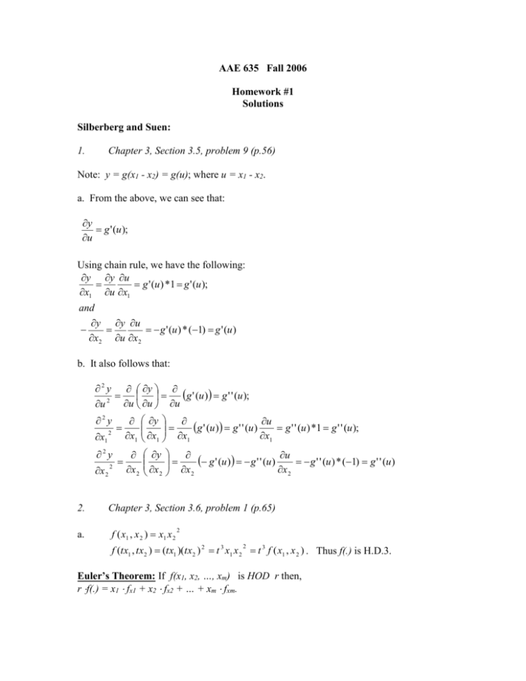
AAE 635 Fall 2006
Homework #1
Solutions
Silberberg and Suen:
1.
Chapter 3, Section 3.5, problem 9 (p.56)
Note: y = g(x1 - x2) = g(u); where u = x1 - x2.
a. From the above, we can see that:
y
 g ' (u );
u
Using chain rule, we have the following:
y y u

 g ' (u ) *1  g ' (u );
x1 u x1
and

y y u

  g ' (u ) * (1)  g ' (u )
x2 u x2
b. It also follows that:
 2 y   y  
g ' (u )  g ' ' (u );

 
u 2 u  u  u
2 y
x1
2
2 y
x 2
2.
a.
2


x1
 y  

 
g ' (u )  g ' ' (u ) u  g ' ' (u ) *1  g ' ' (u );
x1
 x1  x1


x 2
 y

 x 2


 
 g ' (u )    g ' ' (u ) u   g ' ' (u ) * (1)  g ' ' (u )
x 2
 x 2
Chapter 3, Section 3.6, problem 1 (p.65)
f ( x1 , x 2 )  x1 x 2
2
f (tx1 , tx2 )  (tx1 )(tx2 ) 2  t 3 x1 x 2  t 3 f ( x1 , x 2 ) . Thus f(.) is H.D.3.
2
Euler’s Theorem: If f(x1, x2, …, xm) is HOD r then,
r f(.) = x1  fx1 + x2  fx2 + … + xm  fxm.
b.
f
f
2
2
x1 
x 2  x 2 * x1  2 x1 x 2 * x 2  3x1 x 2  3 f ( x1 , x 2 ) , proving that Euler’s
x1
x 2
Theorem holds.
2
f ( x1 , x 2 )  x1 x 2  x 2
f (tx1 , tx2 )  (tx1 )(tx2 )  (tx2 ) 2  t 2 ( x1 x2  x2 )  t 2 f ( x1 , x2 ) . Thus f(. ) is H.D.2.
f
f
2
x1 
x 2  x 2 * x1  x1  2 x 2 * x 2  2 * x1 x 2  x 2  2 f ( x1 , x 2 ) , proving
x1
x 2
that Euler’s Theorem holds.
x  x2
f ( x1 , x 2 )  21
2
x1  2 x 2
tx1  tx2
t( x  x2 )
x  x2
f (tx1 , tx2 ) 
 2 21
 t 1 21
 t 1 f ( x1 , x 2 ) .
2
2
2
2
(tx1 )  2(tx2 )
t ( x1  2 x 2 )
x1  2 x 2
Thus f( ) is H.D. negative 1. Note that this means that as the magnitude of x
increases, f(x) decreases.
2

c.

For notational convenience, let: V  x1  2x 2 .
Then:
f
1
1
2
2
2
2
 2 1* x1  2 x 2  2 x1  x1  x 2   2  x1  2 x 2  2 x1 x 2
x1 V
V
f
1
1
2
2
2
2
 2 1* x1  2 x 2  4 x 2  x1  x 2   2 x1  2 x 2  4 x1 x 2
x 2 V
V
Before proceeding, it is worth noting that:
2
2
3
2
2
3
 1* x1  x 2  x1  2 x 2   x1  2 x1 x 2  x1 x 2  2 x 2
It then follows that:
f
f
1
1
2
2
2
2
x1 
x 2  2  x1  2 x 2  2 x1 x 2 * x1  2 x1  2 x 2  4 x1 x 2 * x 2
x1
x 2
V
V
2
2
 



 












 1* x1  x 2  x1  2 x 2
1
3
2
2
3
 2  x1  2 x1 x 2  x1 x 2  2 x 2 
2
2 2
V
x  2x



 1* x1  x 2 
1
2

2

 1* f ( x1 , x 2 )
2
 2x2
proving that Euler’s Theorem holds.
2
x1
f ( x1 , x 2 ) 
2
x1 x 2  x 2
x
2
1
d.

2
f (tx1 , tx2 ) 

tx1 2

t 2 x1
2

x1
2
 t 0 f ( x1 , x 2 ) .
(tx1 )(tx2 )  (tx2 )
t ( x1 x 2  x 2 ) x1 x 2  x 2
Thus f( ) is H.D.0. Note that this means that if you scale up both x1 and x2 by the
same proportion, the function value remains constant.
2
2
2
2
For notational convenience, let: V  x1 x 2  x 2 .
Then:
x
f
1
2
2
3
2
2
x1  12 2 x1 x1 x 2  x 2  x 2 x1  2 x1 x 2  2 x1 x 2
x1
V
V
2
 






x
f
1
2
3
2
2
x 2  22   x1  2 x 2 x1`  2  x1 x 2  2 x1 x 2
x 2
V
V


It then follows that:
f
f
1
1
3
2
2
3
2
2
x1 
x 2  2 x1 x 2  2 x1 x 2  2  x1 x 2  2 x1 x 2  0 ;
x1
x 2
V
V
proving that Euler’s Theorem holds.

e.



f ( x1 , x 2 )  x1
This implies that:
f (tx1 , tx2 )  tx1  t 1 f ( x1 , x 2 ) , from which we can see that the function is H.D.1.
f
f
x1 
x 2  1* x1  0 * x 2  x1  1* f ( x1 , x 2 ) , proving that Euler’s Theorem
x1
x 2
holds.
NB. The most important “degrees” in economics are the zeroth and the first degree.
However, it is sometimes thought that the Masters and the PhD are even more
important. (Varian, 1992).
3.
Chapter 3, Section 3.6, problem 3 (p.65)

f ( x1 , x 2 )  A x1  1   x 2


 At x


1


  Atx
f (tx1 , tx2 )  A  tx1   1   tx2 

1  1   x 2
Proving that f(. ) is H.D.1.





1
1

 A t  x1  1   t  x 2

1


 1   x 2


1



1

 t * f (tx1 , tx2 )
4. Chapter 5, problem 1 (p. 109). Obtain the inverse of each matrix (if invertible).
(a)
A
1
2
 (3 *1)  (1* 2)  1
1  3
  3 1
Cofactors  C  

 2 1
  3  2
CT  
1 
1
A 1 
1 T 3 2
C 

A
 1  1
check : A 1 A  I
(b)
B
 2 1
 (2) * (3)  (4 * 1)  2
4 3
 3 4 
Cofactors  C  

 1  2
 3 1 
CT  

 4  2
B 1 
  3 / 2 1 / 2
1
; CT  
 1 
B
 2
Check : B 1 B  I
(c )
1
2 1
A 0 1
1 0
1
1
Use the second row for the Laplace expansion;
Note: The value of a determinant |A| of order n can be found by the Laplace expansion of
any row or any column as follows:
n
A   aij | Cij | [Expansion by the i th row]
j 1
n
A   aij | Cij | [Expansion by the j th column]
i 1
A  0
2 1
1 1
1 2
 1*
 1*
0 1
1 1
1 0
 0  0  1(0  2)
 2
| C11 | | C12 | C13 |
Cofactor : C  | C 21 | | C 22 | | C 23 |
| C31 | | C32 | | C33 |
1 1
0 1
0 1
| C11 |
 1; | C12 | 
 1; | C13 |
1
0 1
1 1
1 0
| C 21 | 
| C31 |
2 1
1 1
1 2
 2; | C 22 |
 0; | C 23 | 
 2
0 1
1 1
1 0
2 1
1 1
1 2
 2  1  3; | C32 | 
 1; | C33 |
1
1 1
0 1
0 1
 1 1 1 
 1 2 3 


T
C   2 0  2; C  Adj. A   1 0  1
 3  1 1 
 1  2 1 
  1 / 2 1  3 / 2
CT 
1
A 
  1 / 2 0 1 / 2 
A
 1 / 2 1  1 / 2 
Check : A 1 A  I
(d)
0 1 1
D1 0 1
1 1 0
Using the first row for the Laplace expansion:
0 1
1 1
1 0
D 0
 1*
 1*
1 0
1 0
1 1
 0 11
2
| C11 | | C12 | C13 |
Cofactors : C  | C 21 | | C 22 | | C 23 |
| C 31 | | C 32 | | C 33 |
0 1
1 1
1 0
| C11 |
 1; | C12 | 
 1; | C13 |
1
1 0
1 0
1 1
| C 21 | 
| C 31 |
1 1
0 1
0 1
 1; | C 22 |
 1; | C 23 | 
1
1 0
1 0
1 1
1 1
0 1
0 1
 1; | C 32 | 
 1; | C 33 |
 1
0 1
1 1
1 0
1
1
 1 1
 1 1



T
C   1  1 1 ; C  Adj.D   1  1 1 
 1
 1
1  1
1  1
1/ 2 
 1 / 2 1 / 2
CT 
1
D 
  1 / 2  1 / 2 1 / 2 
D
 1 / 2
1 / 2  1 / 2
Check : D 1 D  I