10/26/99
STT 351-6
HW #5 (Due Th, 11/4) -ANSWERS
1. The present air traffic volume (# landings and takeoffs) at an airport during the peak hour is a normal rv with  = 200
and  = 60 planes.
(a) If the present runway capacity (for traffic) is 350 planes /hr, what is the probability that peak hour traffic produces congestion
(exceeds the capacity of the runway).
P = P[ Z >
350  200
= 2.5] = .0062
60
(b) Assume that in ten years the mean traffic will double, but the sd will only increase to 100.If no additional airports or expansion
is built what would be the probability of congestion 10 years from now?
P = P[ Z >
350  400
= - .5 ] = .6915
100
(c) If the projected growth is correct, what airport capacity will be required in 10 years in order to have the same probability of
congestion as the present one.
C  400
 2 .5  C = 650.
100
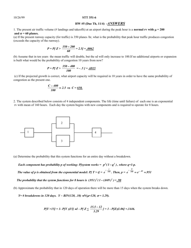
2. The system described below consists of 4 independent components. The life (time until failure) of each one is an exponential
rv with mean of 160 hours. Each day the system begins with new components and is required to operate for 8 hours.
2
1
3
4
zz
zz
z
(a) Determine the probability that this system functions for an entire day without a breakdown.
Each component has probability p of working: P[system works = p 2 ( 1  q 2 ) , where q=1-p.
The value of p is obtained from the exponential model: P[ T > t] = e

t
160
. Then, p = e

8
160
 e  .05  .951
The probability that the system functions for 8 hours is (.951 )2 ( 1  (.049 )2 ) = .90
(b) Approximate the probability that in 120 days of operation there will be more than 15 days when the system breaks down.
Y= # breakdowns in 120 days. Y ~ BIN(120, .10) N(=120,  = 3.29).
P[Y >15] = 1- P[Y 15] 1 - P[ Z <
15 .5  12
] = 1 - P[Z1.06] =.1446.
3 .29
3.
A
C
D
B
6/1
8/1
5/1
The network shown above depicts a sequence of scheduled activities : C can only start after both A and B are completed,
and D starts when A,B, and C are all completed; A,B can go on simultaneously. Each activity has a normal distribution
of completion time:
T(A) ~ N( =25 days,  = 5 days); A starts May 1.
T(B) ~ N( = 26,  = 4)
B starts May 1.
T(C) ~ N( =48,  = 12)
C starts June 1, If A, B are complete.
T(D) ~ N( =40,  =8)
D starts Aug 1, if possible.
For simplicity, assume that all months have 30 days, activity times are all independent. Also, supplies, labor, etc. are such
that if C doesn’t start on time, neither will D.
(a) Determine the probability that activity C will not start on schedule.
1-P = P[T(A)30]P[T(B)30]= P[Z  1]P[Z1]= (.8413 )2 = .708; P = .292
(b) What is the probability that D starts on schedule ?
P = P[both A,B finish by 6/1]P[C finishes by 8/1] = (.708) P[Z  1]=.595.
(c) Given that A is completed by May 1, what is the conditional probability that all activities are completed by August 30?
30  40
P = P[B complete by 6/1]P[C complete by 8/1]P[D complete by 8/30] = (.708)P[Z 
= - 1.25]
8
=(.708)(.1056)=.075.
Note: P[B ok by 6/1, C not complete by 8/1, D ok by 8/30] is negligeable.
4. A company produces two types of items, A, B, both liquid and measured in gallons. Let X denote the daily amount (gals)
of A and let Y denote the daily amount of B produced by the company. Assume:
X ~ N( = 120,  = 12), Y ~ N( = 80,  = 5), Cov(X,Y) = (-24).
Let T=X+Y , the total daily production, and let W=20X + 30Y-1000, the total income ($) from the production of these items.
(a) Determine the means and sd’s of (i) T and (ii) W
(i) E(T) = 120+80=200. Var(T) = 144+25 + 2 (-24)=121; SD(T)=11.
(ii) E(W)=(20 120) + (30 80) - 1000=3800. Var(W)=400 144+900 25 - 2 20 30 24=51,300; SD(W)=226.5
(b) Obtain (i) P[W > 5000]; (ii) the 90 th percentile of W.
(i) P[W>5000]=P[Z>
5000  3800
=5.3]  0. (ii) 90th %ile of Z is 1.2890th %ile of W is 3800+226.5(1.28)4090.
226 .5
(c) Determine the probability that on a given day, the amount of A produced is more than twice that of B.
P[X>2Y] = P[X-2Y>0]. E(X-2Y)=120-160= - 40; Var(X-2Y) = 144+4 25 - 2 2 (-24)= 340; SD(X-2Y) = 18.44.
40
P[X-2Y>0]=P[Z>
= 2.17] = .015
18 .44
5. Both east and west bound rush-hour traffic on a toll bridge were counted at 10 second intervals. The results are given in the
following table: The entries give the number of 10-sec intervals that had i east-bd and j west-bd vehicles. Altogether there were
400 observations.
0
0
1
X=#E-B Vehs 2
3
pY
Y=#W-B Vehs
1
2
3
.005
.0125
.040
.1125
.015
.020
.070
.075
.035
.0675
.100
.0775
.125
.100
.100
.045
.17
.18
.28
.37
pX
.18
.20
.31
.31
(a) Convert the table to a joint probability function of X and Y (DONE - divided each entry by 400)
(b) Determine the marginal pmf's of X and Y, respectively. (Exhibited in the margins of the table)
(c) Obtain the conditional pmf of Y given X=3. (Divide each entry in the row [X=3] by .31.
y
0
1
2
3
P[Y=y|X=3]
.36 .24 .25
.15
(d) Given that there are 3 vehicles going west in a given 10-sec interval, what is the conditional probability that there are also 3
vehicles going east?
P[X=3 | Y=3] = .045/.37 = .12.
(e) Determine the correlation, (X,Y). 1st obtain means and sd's from the marginals:
E(X) = 1.75, Var(X) = 4.23- 175
. 2 =1.17, SD(X) = 1.08.
E(Y) = 1.85, Var(Y) = 4.63- 1.85 2 =1.21, SD(Y) = 1.10.
E(XY): In cell i-j obtain the product i  j P[X=i,Y=j], then sum over all cells:( 1st row, 1st column - all 0's)
E(XY) = .020(1)+.0675(2)+.100(3) +.070 (2)+.100(4)+.100(6) +.075 (3)+.0775(6)+.045(9) = 2.69.
Hence Cov(X,Y) = 2.69 - (1.75)(1.85) = -.55 and Corr(X,Y) = (X,Y) = -.55/(1.08)(1.10) = - .46.
6. The joint density of X and Y is given by: f(x,y) = e  x , 0  y  x <  and 0, elsewhere.
(a) Sketch the region in the x-y plane where f is positive.
y
y>x
y  x: f is positive here.
x
(b) Determine the marginals of X and Y :
x

0
y
z
z
Marginals: f X ( x )  e  x dy  xe  x , x  0 (Gam(2,1)); fY ( y )  e  x dx  e  y , y  0 (Exp(1) =Gam(1,1)).
(c) Determine (and name) the conditional distribution of Y given X=x.
f ( x, y )
ex
1
fY ( y| X  x ) 

 , 0  y  x.
fX ( x )
x
xe  x
The conditional distribution of Y given X=x is Uniform on the interval [0, x].
(d) From the marginals: E(X) = 2=Var(X), SD(X) = 1.41; E(Y)=1=Var(Y)=SD(Y).

x
 x3
1
= .71.
E( XY )  [ xe  x ydy ] dx 
e  x dx  3 . Cov(X,Y) = 3-(2)(1) = 1. (X,Y) =
1.41
0
0
0 2
z
z
z
(c) Determine (and name) the conditional distribution of Y given X=x.
(d) Determine (X,Y).
f(x,y) = e  x , 0  y  x <  .
x

0
y
z
z
Marginals: f X ( x )  e  x dy  xe  x , x  0 (Gam(2,1)); fY ( y )  e  x dx  e  y , y  0 (Exp(1) =Gam(1,1)).
2. Modify #52 in Ch 5: Answer the questions using the model of #46.
(a) X,Y not exchangeable. They have different marginals and f(x,y)  f(y,x).
(b) Marginals given in #1. (c) E(X) = 1 = Var(x); E(Y) = 2 = Var(Y). Then,  X Y  2
(d) Not independent. f > 0 only on {(x,y) : 0 < x< y}. This is enough to preclude independence.
y

 y3
1
e  y dy  3  Cov(X,Y) = 3-2 = 1 and  =
(e) E( XY )  [ ye  y xdx ] dy 
.
0
0
0 2
2
z z
3. Ch 5, #63. (a) fY ( y| X  x ) 

(c) E(Y) =
zy e
2 y
z
e y
 e _( y  x ) , y  x .
ex

z
(b) E(Y|X=x) = e x ye  y dy ( 1  x ) .
x
dy =2 (from marginal) and Var(Y) = 2, also.
0
Since E(X) = 1 and E(Y|X)=1+X, it follows that E(E(X|Y))= 1 + E(X) = 2.
(d) Also, Var(Y|X) = 1 (The cond dist of Y given X=x is that of X* + x, where X* is an exponential rv).
Var(E(Y|X)) = Var(1+X) = Var(X)=1. Hence, E(Var(Y|X)) + Var(E(Y|X))= 1+1=2, as given in (c).