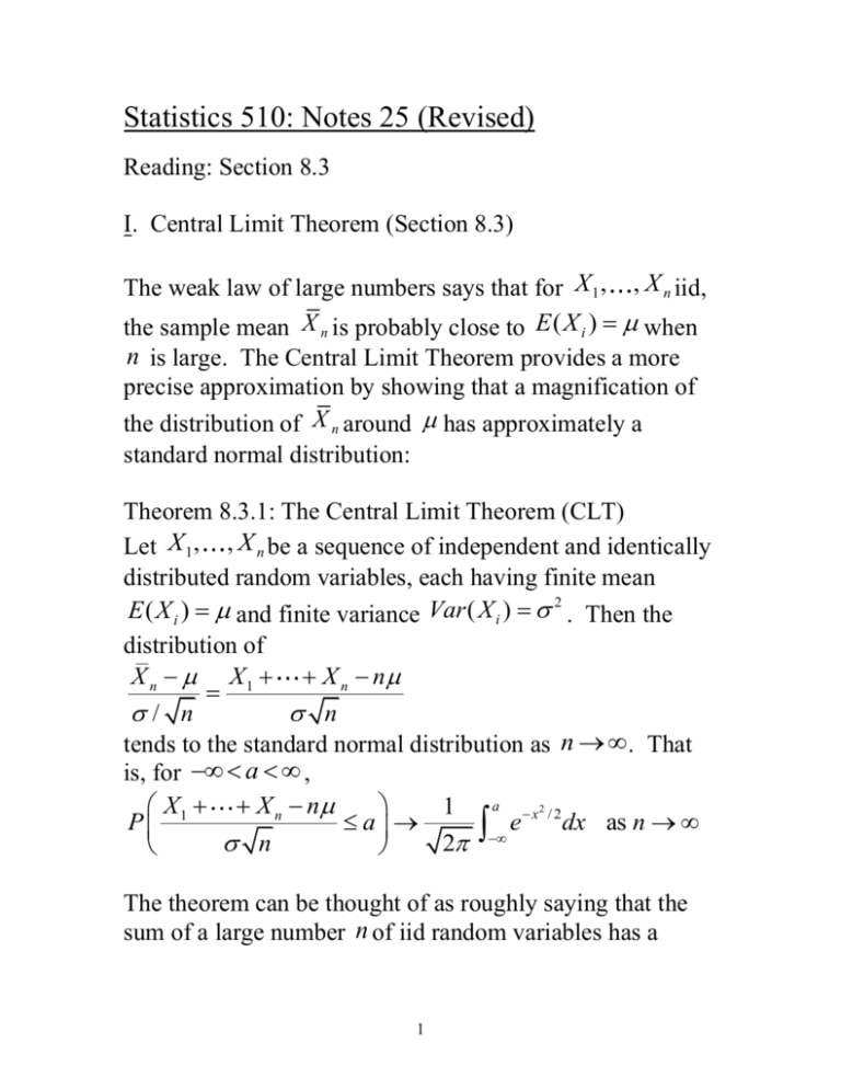
Statistics 510: Notes 25 (Revised)
Reading: Section 8.3
I. Central Limit Theorem (Section 8.3)
The weak law of large numbers says that for X 1 , , X n iid,
the sample mean X n is probably close to E ( X i )   when
n is large. The Central Limit Theorem provides a more
precise approximation by showing that a magnification of
the distribution of X n around  has approximately a
standard normal distribution:
Theorem 8.3.1: The Central Limit Theorem (CLT)
Let X 1 , , X n be a sequence of independent and identically
distributed random variables, each having finite mean
E ( X i )   and finite variance Var ( X i )   2 . Then the
distribution of
X n   X 1   X n  n

/ n
 n
tends to the standard normal distribution as n   . That
is, for   a   ,
1 a  x2 / 2
 X   X n  n

P 1
 a 
e
dx as n  


 n
2


The theorem can be thought of as roughly saying that the
sum of a large number n of iid random variables has a
1
distribution that is approximately normal with mean
n and variance n 2 . By writing
X1   X n
1  X   X  n 

1
n
X 1   X n  n
n
 n


1  n
 n
n
n
we see that the CLT says that the sample mean
X   Xn
Xn  1
has a approximately a normal
n
distribution with mean  and variance  .


n
The CLT is a remarkable result – only assuming that a
sequence of iid random variables have a finite mean and
variance, the central limit theorem shows that the mean of
the sequence, suitably standardized, always converges to
having a standard normal distribution.
Note: The normal approximation to the binomial
distribution from Section 5.4.1 is a special case of the
central limit theorem.
Before examining the proof, we look at a few applications.
Example 1: Do you believe a friend who claims to have
tossed heads 5,250 times in 10,000 tosses of a fair coin?
2
Example 2: Bill makes 100 check transactions between
receiving two consecutive bank statements. Rather than
subtract each amount exactly, he rounds each entry off to
the nearest dollar. Let X i denote the round-off error
associated with the i th transaction [it can be assumed that
X i has a uniform distribution over the interval (-0.5,0.5)].
Use the central limit theorm to approximate that Bill’s total
accumulated error (either positive or negative) after 100
transactions exceeds $5.
3
4
Proof of the Central Limit Theorem
We know from Chapter 7.7 that a distribution function is
uniquely determined by its moment generating function.
The following lemma states that this unique determination
holds for limits as well (see W. Feller, An Introduction to
Probability Theory and Its Applications, Volume II, 1971,
for the proof)
Lemma 8.3.1: Let Z1 , Z 2 ,
be a sequence of random
variables having distribution functions FZ n and moment
generating functions M Z n , n  1 ; and let Z be a random
variable having distribution function FZ and moment
generating function M Z . If M Z n (t )  M Z (t ) for all t, then
FZ n (t )  FZ (t ) for all t at which FZ (t ) is continuous.
If we let Z be a standard normal random variable, then, as
M Z (t )  e
t2 / 2
, it follows from Lemma 8.3.1, that if
t 2 / 2
as n   , then FZn (t )  (t ) as n   .
The central limit theorem is proved by showing that the
moment generating functions of
X 1   X n  n
M Zn (t )  e
 n
converge to e
t2 / 2
as n   .
Proof of central limit theorem: We shall prove the theorem
under the assumption that the moment generating function
5
*
of the X i , M X (t ), exists and is finite. Let X i 
Xi  

.
Note that
t
E ( X i* )  0, Var( X i* )  1, M X * (t )  e  t /  M X 

X 1* ,

.

, X n* are independent so that the moment generating
*
function of X 1 
M (t )   M X *  t  
 X n* is
n
and the moment generating function of
X   X n  n
1
Zn  1

( X 1*   X n* )
 n
n
is
n

 t 
M Z n (t )   M X * 
 .
n



Let L(t )  log M X * (t ) . To prove the theorem, we much
2
show that M Zn (t )  t / 2 as n   or equivalently that
 t 
2
log M Zn (t )  nL 

t
/2

n


as n   .
To show this, note that
6
lim n
L(t /( n ))
tn 3/ 2 L '(t /( n ))
 lim n
(by L'Hopital's rule)
1/ n
2n 2
tL '(t / n )
n 1/ 2
t 2 n 3/ 2 L ''(t / n ))
 lim n
(by L'Hopital's rule)
2n 3/ 2
 lim n
 lim n
t 2 L ''(t /( n ))
2
Note further that
L(0)  0
M '(0)
L '(0) 
 M '(0)  E ( X * )  0
M (0)
M (0) M ''(0)  [ M '(0)]2
* 2
L ''(0) 

E
((
X
) ) 1
2
[ M (0)]
Thus,
lim n
L(t / n ))
t 2 L ''(t / n ))
 lim n
1/ n
2
t2

,
2
which proves that M Z n (t )  e as n   and hence that
FZn (t )  (t ) by Lemma 8.3.1.
t2 / 2
How large does n need to be for the CLT to provide a good
approximation?
7
For practical purposes, especially for statistics, the limiting
result in the CLT is not of primary interest. Statisticians
are more interested in its use as an approximation with
finite values of n. It is impossible to give a concise and
definitive statement of how good the approximation is, but
some general guidelines are available, and examining
special cases can give insight. How fast the approximation
becomes good depends on the distribution of the X i ’s. If
the distribution is fairly symmetric and has tails that die off
rapidly, the approximation becomes good for relatively
small values of n. If the distribution is very skewed or if
the tails die down very slowly, a larger value of n is needed
for a good approximation.
Example 3: Since the uniform distribution on (0,1) has
mean 1 and variance 1 , the sum of 12 uniform random
2
12
variables, minus 6, has mean 0 and variance 1. The central
limit theorem says that the distribution of this sum is
approximately standard normal and in fact the distribution
is quite close to the standard normal. In fact, before better
algorithms were developed, the sum of 12 uniform random
variables minus 6 was commonly used in computers for
generating normal random variables from uniform ones.
8
Example 4: Dice rolls. Let X 1 , X 2 , be independent and
identically distributed rolls of a die that has probability
mass function
P( X i  1)  p1 , P( X i  2)  p2 , P( X i  3)  p3 ,
P( X i  4)  p4 , P( X i  5)  p5 , P( X i  6)  p6
The charts attached to this note show histograms of the
probability distribution for the sums X 1   X n for
n  5,10,15, 20 rolls of the die for
(1) the unbiased die with the symmetrical distribution
1
p1  p2  p3  p4  p5  p6 
6
(2) the biased die with the asymmetrical distribution
p1  0.2, p2  0.1, p3  0.0, p4  0.0, p5  0.3, p6  0.4
9
It is quite apparent that for both distributions (1) and (2) of
the die, the distribution of the sums X 1   X n is
approximately a normal (bell-shaped) distribution by
n  20 , but the sums take on an approximately normal
distribution earlier for the symmetric distribution (1) than
for the asymmetric distribution (2).
The speed of convergence of the distribution of the sample
mean to its limiting distribution for different distributions is
also illustrated by the applet at
http://www.ruf.rice.edu/~lane/stat_sim/sampling_dist/index
.html .
10