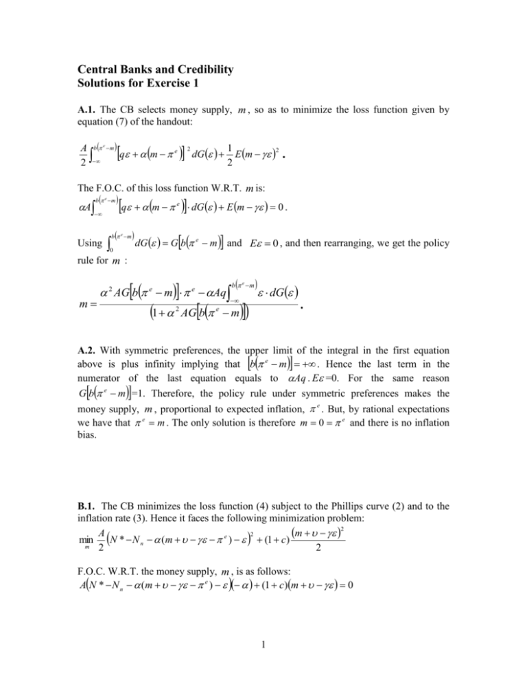
Central Banks and Credibility
Solutions for Exercise 1
A.1. The CB selects money supply, m , so as to minimize the loss function given by
equation (7) of the handout:
A b  e m 
q   m   e



2



2
dG   
1
2
E m    .
2
The F.O.C. of this loss function W.R.T. m is:
b  e  m 
A
q   m   e   dG    E m     0 .


Using



b  e m
0



dG    G b e  m  and E  0 , and then rearranging, we get the policy
rule for m :
 AGb  m   Aq 
2
m
e
1  
e
2


b  e m

AG b  e  m


  dG 
.
A.2. With symmetric preferences, the upper limit of the integral in the first equation
above is plus infinity implying that b  e  m   . Hence the last term in the
numerator of the last equation equals to Aq . E =0. For the same reason
G b  e  m =1. Therefore, the policy rule under symmetric preferences makes the
money supply, m , proportional to expected inflation,  e . But, by rational expectations
we have that  e  m . The only solution is therefore m  0   e and there is no inflation
bias.




B.1. The CB minimizes the loss function (4) subject to the Phillips curve (2) and to the
inflation rate (3). Hence it faces the following minimization problem:
2
m     2
A
min N *  N n   (m       e )     (1  c)
m
2
2
F.O.C. W.R.T. the money supply, m , is as follows:
AN *  N n   (m       e )       (1  c)m       0
1
Rearranging to solve for the money supply, m , we get the reaction function of the CB:


A
2A
2A
N *  N n      
m

e.

2
2
2
1 c  A
1 c  A 
1 c  A







B.2. By rational expectations we have that:
 e  E  E (m     )  Em .
Substituting the Central-Bank reaction function, we get
1
e 
A ( N *  N n )  A 2 e
2
1  c  A


e 
A ( N *  N n )
1 c

.
B.3. First, let's substitute the expected inflation,  e , into the CB reaction function, to get:
m


A
2A

N *  N n      
2
1  c 
1  c   A .

Now, substitute the last expression in the Phillips curve:
A
A
  m     
(N * Nn ) 
 .
1 c
1  c  A 2
And, finally, substitute the last expression in the expression for actual employment,
equation (2), to get:
1 c
N  N n      e     N n 
.
1  c  A 2
The last two equations are the expressions for inflation and employment, in terms of
exogenous variables and the shocks.
B.4. Substituting actual inflation and employment (the last two expressions) into the
society loss function (1), we obtain:
A
2
2
Loss  N *  N  

2
2
A
1 c
A
 1  A

  
(N * Nn ) 
 .
 N * Nn 
2
2
2
2
1

c
1  c  A 
1  c  A 

2
2
Since the unconditional expected value of the shock  is zero. Thus, expressions
including its first moment are dropped. The expected society loss, therefore, becomes:
2
2
A
A 2 
A  1  c   A 2  2
2
 N *  N n   
Loss  1 


2  1  c 2  
2  1  c  A 2 2 

S

 

Ks
 Loss 
K
A
K s 2  K  2  .
2 s
B.5. Since the shock  appears only in the expression for inflation, it doesn't induce
output-inflation tradeoff (as opposed to the other shock,  ). Hence the optimal
discretionary policy fully offsets the impact of this shock on inflation, as can be seen by
the policy rule in the answer to question (1) above. As a result, the inflation expression in
the answer to question 3 above doesn't include this shock either. As a result, the variance
of  does not cause any welfare losses.
B.6. While both terms are positive, the partial derivatives are:
K s
2 A 2

0 .
c
1  c 3
K
2 A 2 c

0 .
c
1  c  A 2 3
The fact that both K s and K  are positive means that both quadratic terms are welfare
reducing. However, as we see by the derivatives, the more we increase the CB
conservativeness, c , the more we decrease the welfare loss attributed to unemployment
deviations, s 2 , but at the same time the more we increase the welfare loss attributed to
the shock  2 . It follows that there is some finite level of c , for which losses attributed to
both sources are at the same level. This would be the optimal level of CB conservatism.
B.7. The derivative of society loss function with respect to c given is by the following
expression:





L A  2 A 2 2
2 A 2 c
A
2 A 2 c

2
2 2
2
 
s 
 
 2 A s 
 
3
c 2  1  c 3
1  c  A 2 3  21  c 3 

A 2 

1 



1

c




Hence the F.O.C. is as follows
3
L
2 A 2 c
 0  2 A 2 s 2 
2 0
3
c

A 2 
1 

 1 c 
One can see that when c = 0 the right hand side of this expression is always negative.
When c   , the right hand side goes to infinity as well. Hence, there has to be c that
solves this problem, and it will be higher than zero and finite.
B.8. First note that in the last derivative, the right term is a positive function of c , since
c increases the nominator and decreases the denominator. Now note that s 2 increases
with the employment target, N * , and therefore the left term grows more negative. That
means the c has to increase so as to counterbalance it. At the same time, when  2
increases, the right term grows more positive, and c has to fall so as to counterbalance it.
4